
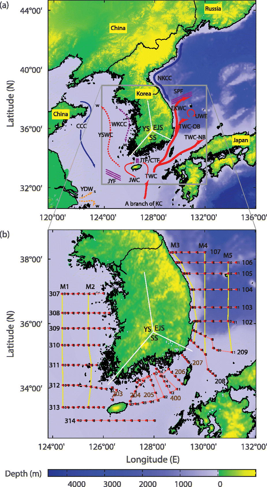
Fig. 1.
(a) Schematic regional circulation around the Korean Peninsula. Blue, red, purple, and orange colors indicate the water temperature of cold, warm, fronts, and riverine waters, respectively. Solid and dashed curves denote the persistent and seasonal currents, respectively ( and indicate the directions of currents in summer and winter, respectively). Acronyms of primary regional currents are listed in the order of the Yellow Sea (YS), South Sea (SS), and East/Japan Sea (EJS): Yellow Sea Warm Current (YSWC), West Korea Coastal Current (WKCC), Chinese Coastal Current (CCC), Jeju Warm Current (JWC), Jeju Tsushima Front (JTF)/Cheju Tsushima Front (CTF), Jeju Yangtze Front (JYF), Yangtze Diluted Water (YDW), Kuroshio Current (KC), North Korea Cold Current (NKCC), Tsushima Warm Current (TWC), Tsushima Warm Current-Nearshore Branch (TWC-NB), Tsushima Warm Current-Offshore Branch (TWC-OB), East Korea Warm Current (EKWC), Subpolar Front (SPF), and Ulleung Warm Eddy (UWE) (see Table 1 for more details). (b) Historical hydrographic survey lines and stations for conductivity-temperature-depth (CTD) profiles for a period of recent 20 years (1995 to 2014) are marked with red lines and black dots, respectively. Three sub-regions are divided into the YS (Lines 307 to 314), SS (Lines 400, and 203 to 207), and EJS (Lines 102 to 107, 208, and 209) regions. CTD stations at each line are numbered with from 0 to 11, corresponding to nearshore to offshore regions except for stations on Line 400 (12th to 27th stations). Five meridional lines ( to ) are marked with yellow lines.
Table 1.
Acronyms and full names of the regional currents and water masses around the Korean Peninsula are listed as a regional order (YS, SS, and EJS) and an alphabetical order.
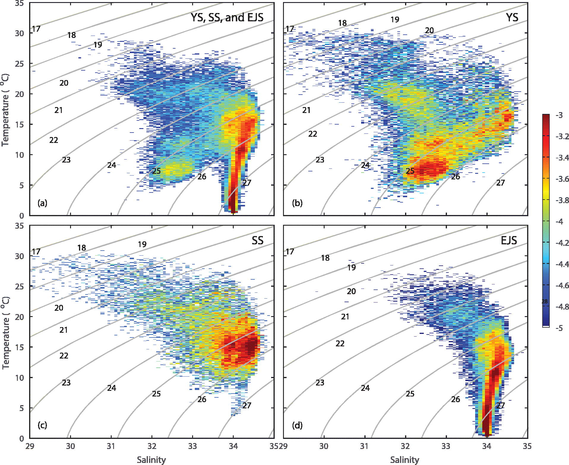
Fig. 2.
Joint probability density functions ( scale) of the available temperature and salinity data at all depths for a period of recent 20 years (1995 to 2014) in the entire domain and three regions of the YS, SS, and EJS are overlaid with T/S diagrams. Bin sizes of the temperature and salinity are equal to 0.08°C and 0.08, respectively. Gray contours denote the density anomalies (). (a) Entire domain. (b) YS (Lines 307 to 314). (c) SS (Lines 400 and 203 to 207). (d) EJS (Lines 102 to 107, 208, and 209).
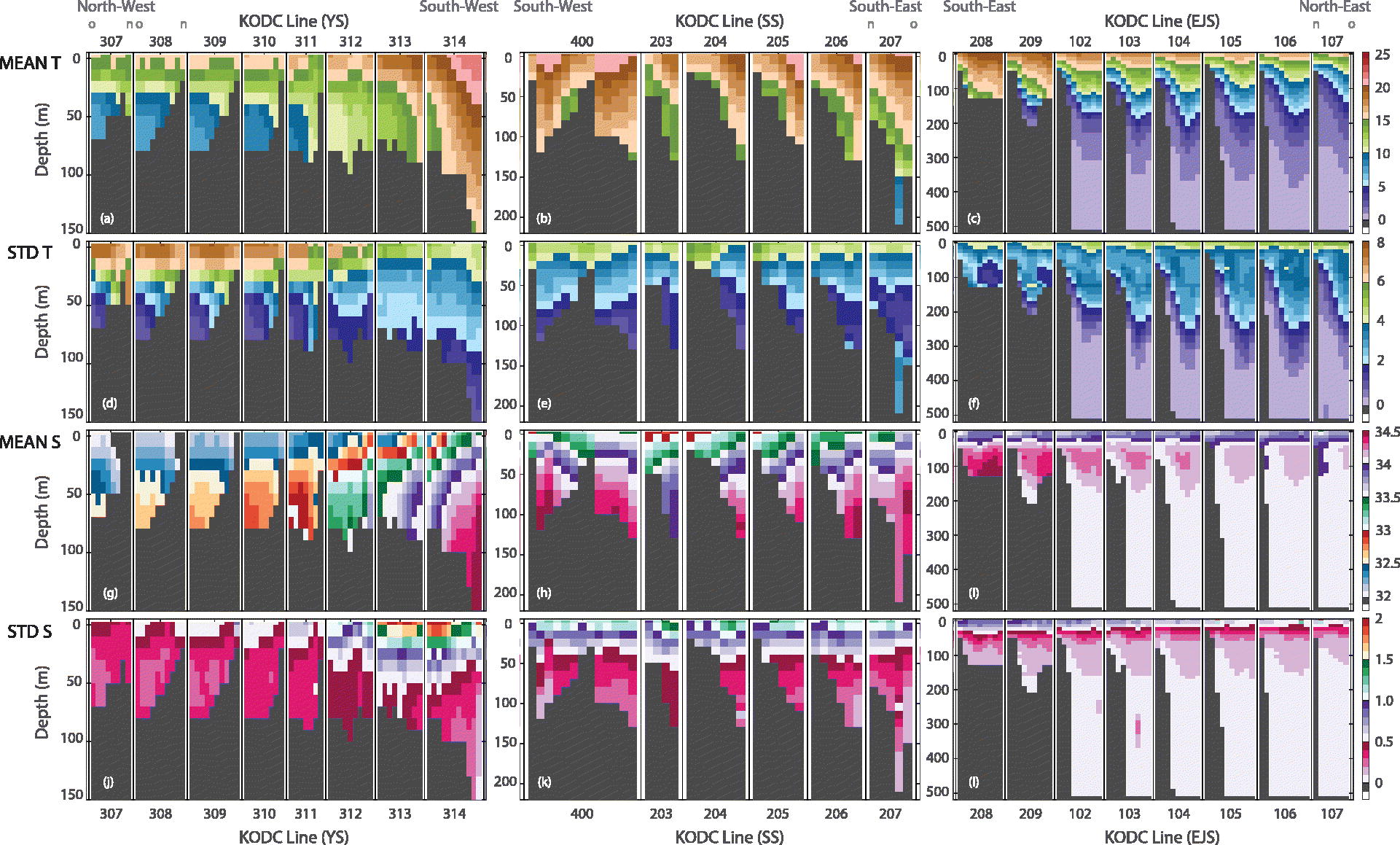
Fig. 3.
Zonal sections of the temporal mean () and standard deviation () of the temperature (C) and salinity profiles sampled in the YS, SS, and EJS for a period of recent 20 years (1995 to 2014). (a–c) Temporal mean of the temperature. (d–f) Standard deviation of the temperature. (g–i) Temporal mean of the salinity. (j–l) Standard deviation of the salinity. (a), (d), (g), and (j): YS. (b), (e), (h), and (k): SS. (c), (f), (i), and (l): EJS. The vertical profiles are concatenated in terms of cross-shore lines, and the unsampled depths and bottom bathymetry are shown as gray columns.
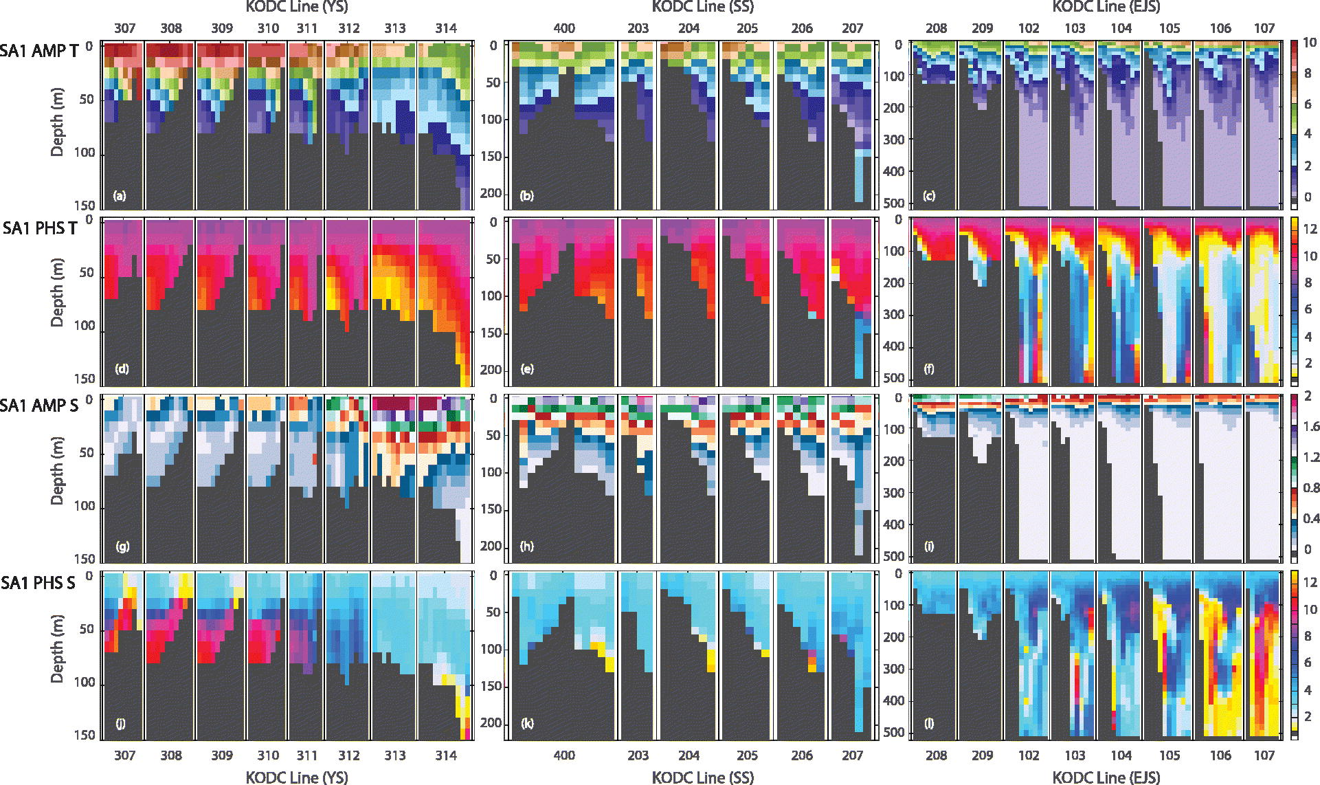
Fig. 4.
Zonal sections of the annual amplitudes and phases (SA1) of the temperature (C) and salinity profiles sampled in the YS, SS, and EJS for a period of recent 20 years (1995 to 2014). (a–c) Annual amplitudes of the temperature. (d–f) Annual phases of the temperature. (g–i) Annual amplitudes of the salinity. (j–l) Annual phases of the salinity. (a), (d), (g), and (j): YS. (b), (e), (h), and (k): SS. (c), (f), (i), and (l): EJS. The vertical profiles are concatenated in terms of cross-shore lines, and the unsampled depths and bottom bathymetry are shown as gray columns. The phase is converted into the month of the year.
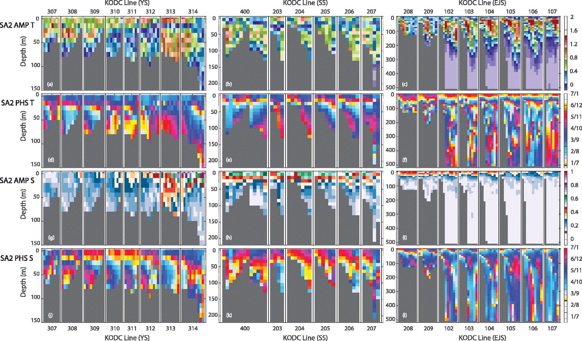
Fig. 5.
Zonal sections of the semi-annual amplitudes and phases (SA2) of the temperature (C) and salinity profiles sampled in the YS, SS, and EJS for a period of recent 20 years (1995 to 2014). (a–c) Semi-annual amplitudes of the temperature. (d–f) Semi-annual phases of the temperature. (g–i) Semi-annual amplitudes of the salinity. (j–l) Semi-annual phases of the salinity. (a), (d), (g), and (j): YS. (b), (e), (h), and (k): SS. (c), (f), (i), and (l): EJS. The vertical profiles are concatenated in terms of cross-shore lines, and the unsampled depths and bottom bathymetry are shown as gray columns. The phase is converted into the month of the year.
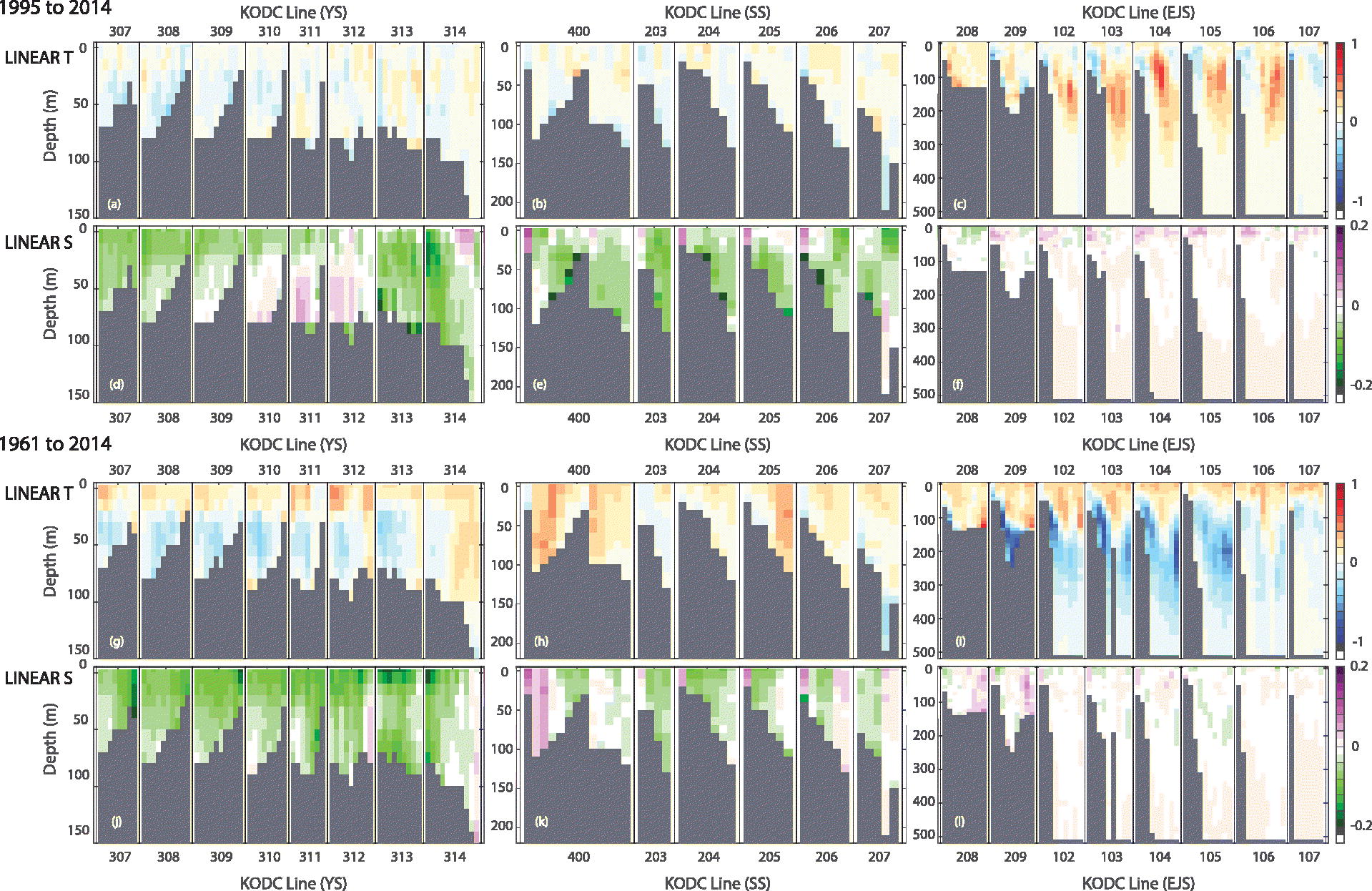
Fig. 6.
Zonal sections of the linear trend of the temperature (C) and salinity profiles sampled in the YS, SS, and EJS for a period of recent (a–f) 20 years (1995 to 2014) and (g–l) 54 years (1961 to 2014). The linear trend is presented as the value for 10 years. (a–c) Linear trend of the temperature. (d–f) Linear trend of the salinity. (g–i) Linear trend of the temperature. (j–l) Linear trend of the salinity. The vertical profiles are concatenated in terms of cross-shore lines, and the unsampled depths and bottom bathymetry are shown as gray columns.
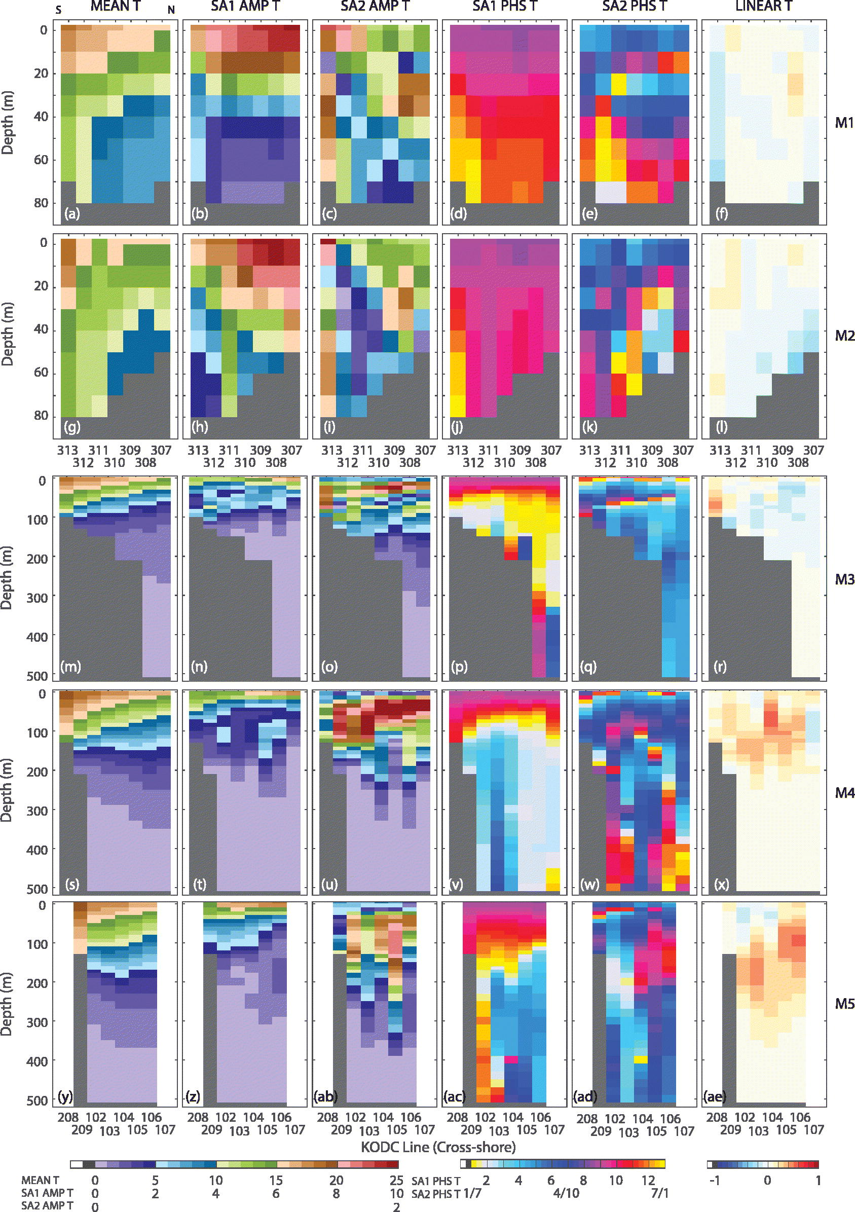
Fig. 7.
Meridional sections of the temporal mean, amplitudes and phases at the annual and semi-annual frequencies, and linear trend of the temperature in the YS ( and ) and EJS ( and ). (a), (g), (m), (s), and (y): Temporal mean of the temperature. (b), (h), (n), (t), and (z): Annual amplitudes of the temperature (SA1). (c), (i), (o), (u), and (ab): Annual phases of the temperature (SA1). (d), (j), (p), (v), and (ac): Semi-annual amplitudes of the temperature (SA2). (e), (k), (q), (w), and (ad): Semi-annual phases of the temperature (SA2). (f), (l), (r), (x), and (ae): Linear trend of the temperature. (a–f) (g–l) (m–r) (s–x) (y–ae) The linear trend of the temperature is presented as the value for 10 years. The vertical profiles are concatenated in terms of cross-shore lines, and the unsampled depths and bottom bathymetry are shown as gray columns. The phase is converted into the month of the year.
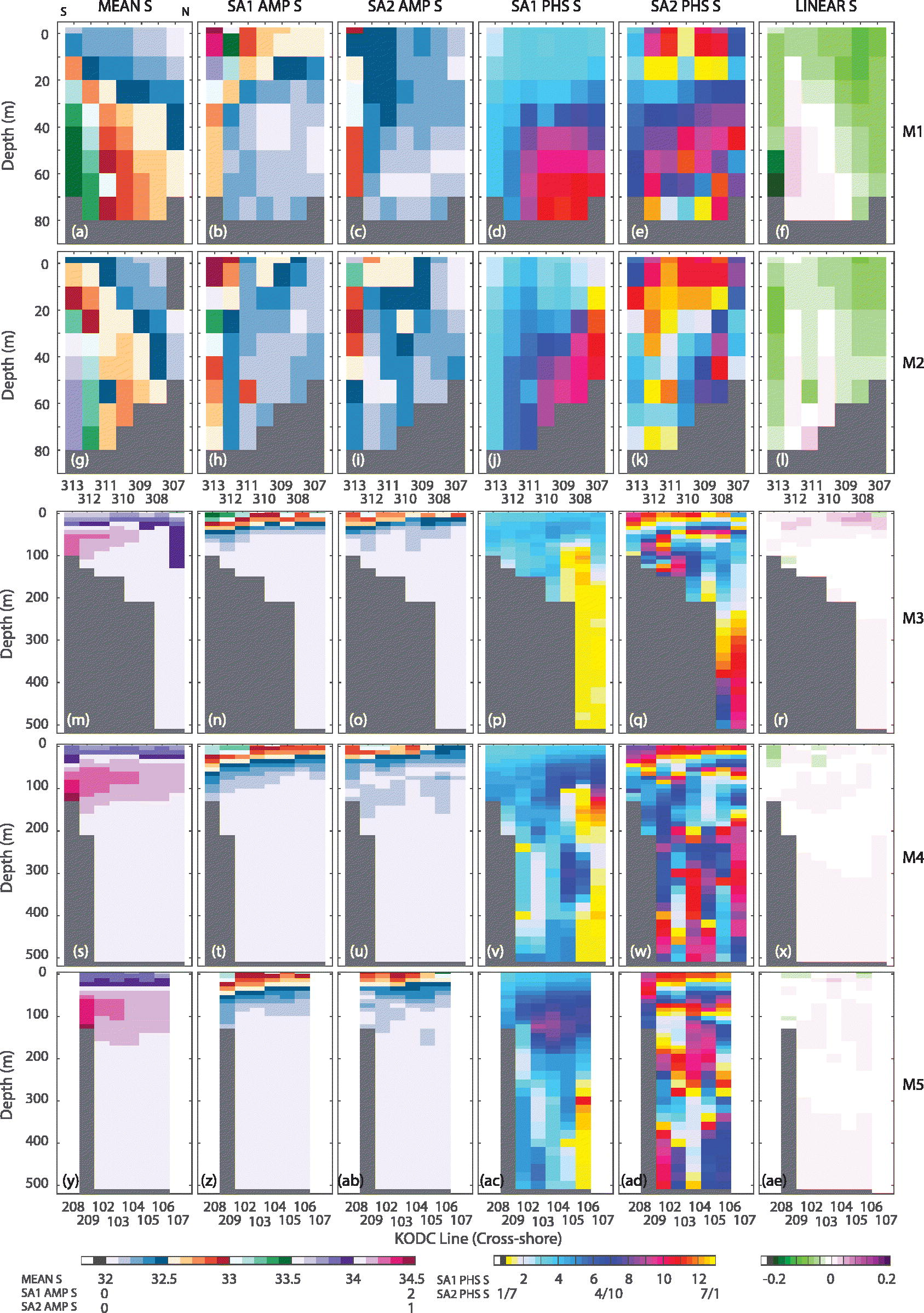
Fig. 8.
Meridional sections of the temporal mean, amplitudes and phases at the annual and semi-annual frequencies, and linear trend of the salinity in the YS ( and ) and EJS ( and ). (a), (g), (m), (s), and (y): Temporal mean of the salinity. (b), (h), (n), (t), and (z): Annual amplitudes of the salinity (SA1). (c), (i), (o), (u), and (ab): Annual phases of the salinity (SA1). (d), (j), (p), (v), and (ac): Semi-annual amplitudes of the salinity (SA2). (e), (k), (q), (w), and (ad): Semi-annual phases of the salinity (SA2). (f), (l), (r), (x), and (ae): Linear trend of the salinity. (a–f) (g–l) (m–r) (s–x) (y–ae) The linear trend of the salinity is presented as the value for 10 years. The vertical profiles are concatenated in terms of cross-shore lines, and the unsampled depths and bottom bathymetry are shown as gray columns. The phase is converted into the month of the year.
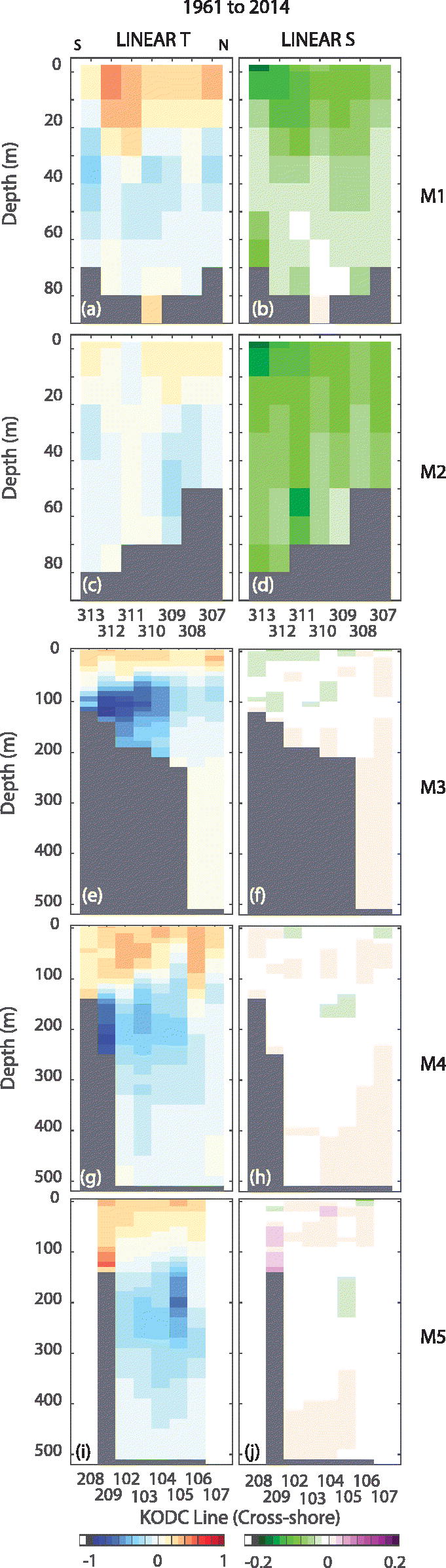
Fig. 9.
Meridional sections of the linear trend of the temperature and salinity in the YS ( and ) and EJS ( and ) for a period of 54 years (1961 to 2014). (a), (c), (e), (g), and (i): Linear trend of the temperature. (b), (d), (f), (h), and (j): Linear trend of the salinity. (a) and (b): (c) and (d): (e) and (f): (g) and (h): (i) and (j): The linear trend of the salinity is presented as the value for 10 years. The vertical profiles are concatenated in terms of cross-shore lines, and the unsampled depths and bottom bathymetry are shown as gray columns.
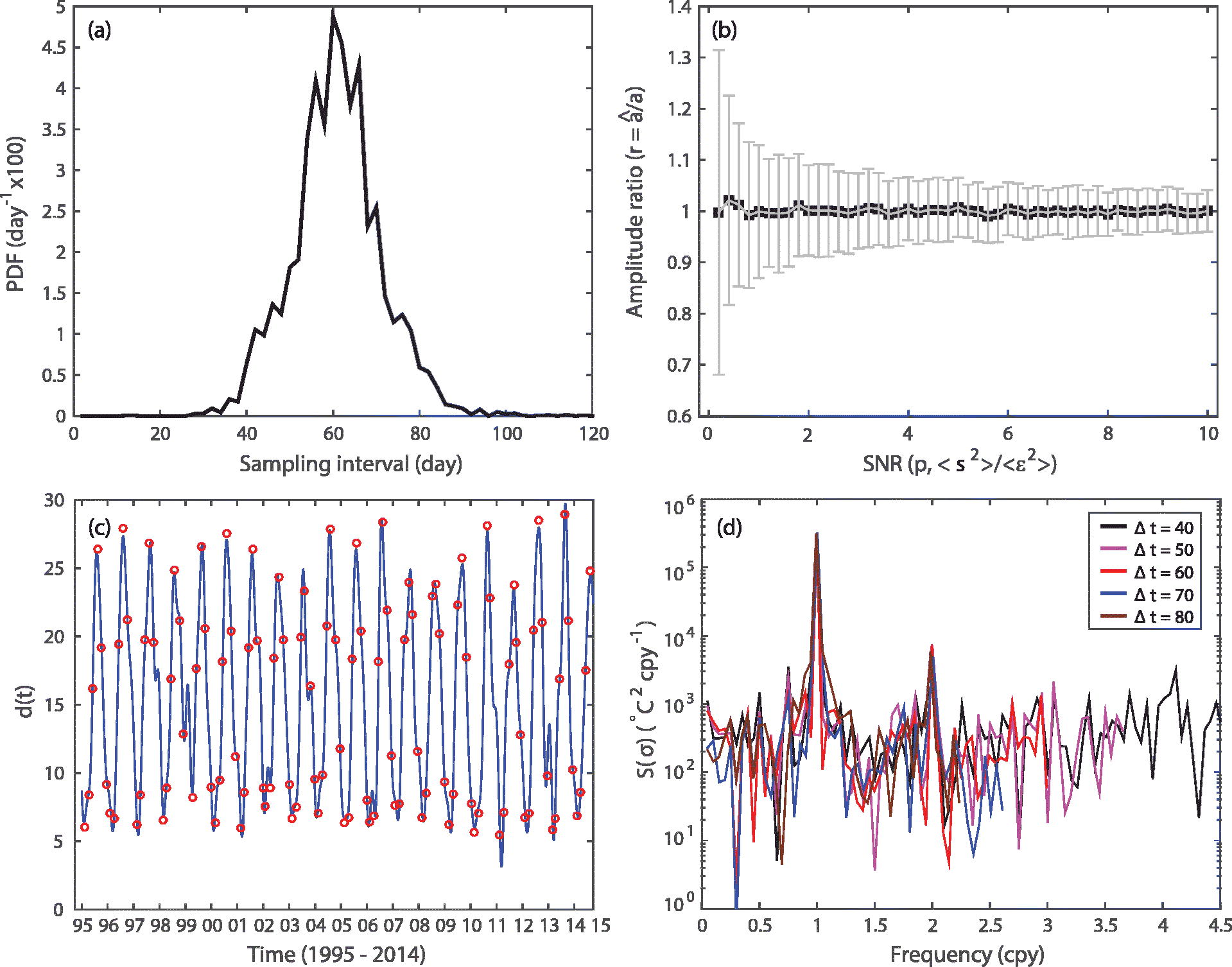
Fig. A1.
(a) A PDF of sampling intervals obtained from the CTD data for a period of recent 20 years (1995 to 2014). (b) Ensemble mean of ratios () of the estimated amplitude () to true amplitude (a in Equation A2) is presented as a function of SNR () in Equation A4). (c) Reconstructed temperature time series (blue) and sampled data (red circles) at the Line 307, station 10, and 0 m depth when the time axis is defined with days. (d) Energy spectra of reconstructed temperature time series using the slow FFT method are presented as a function of constant time intervals ( 40, 50, 60, 70, and 80 days). The noise floor level is equal to 1.78C, and the frequency axis is given as cycles per year (cpy).
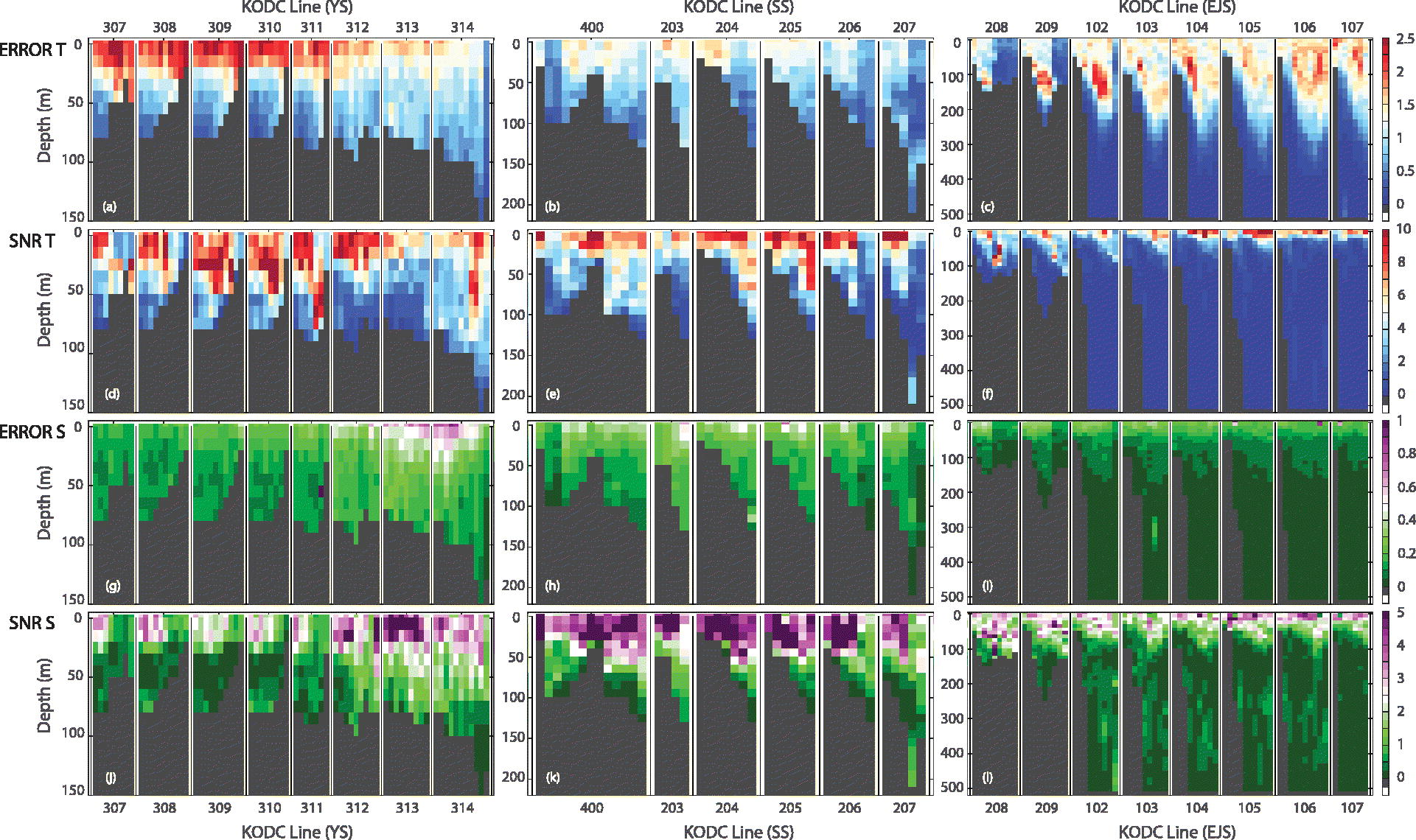
Fig. A2.
Zonal sections of the observational noise (ϵ) and SNR (p) of the temperature (C) and salinity profiles at the annual frequency () sampled in the YS, SS, and EJS for a period of recent 20 years (1995 to 2014). (a–c) Observational noise (ϵ) of the temperature at the annual frequency. (d–f) SNR (p) of the temperature at the annual frequency. (g–i) Observational noise (ϵ) of the salinity at the annual frequency. (j–l) SNR (p) of the salinity at the annual frequency. (a), (d), (g), and (j): YS. (b), (e), (h), and (k): SS. (c), (f), (i), and (l): EJS. The vertical profiles are concatenated in terms of cross-shore lines, and the unsampled depths and bottom bathymetry are shown as gray columns.
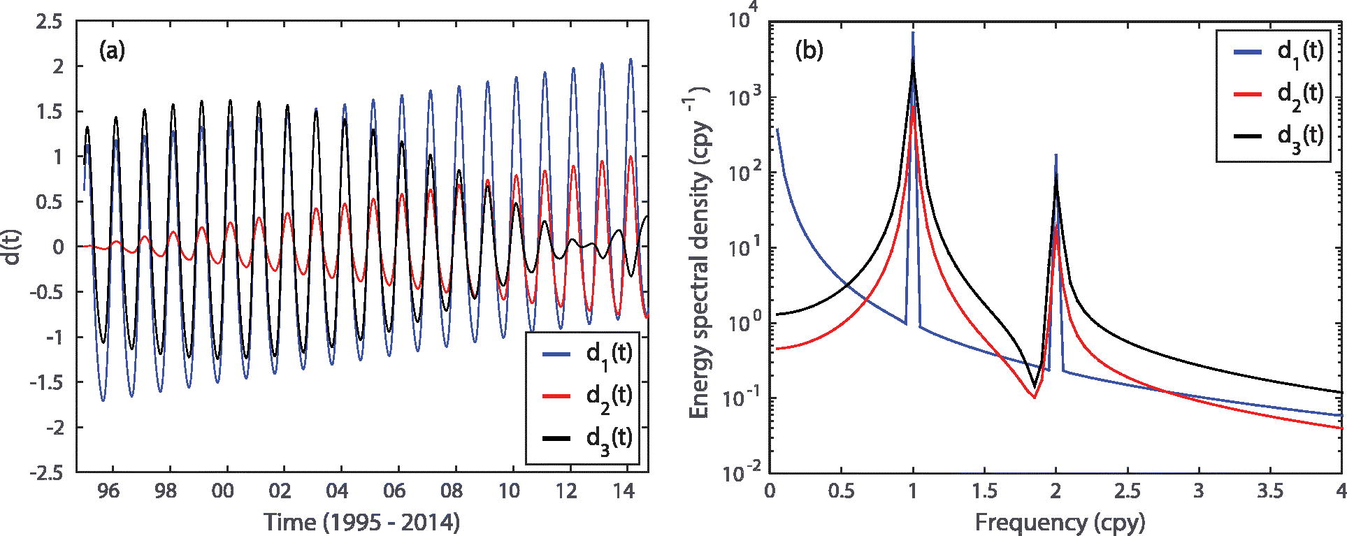
Fig. C1.
(a) Examples of time series modulated with linear sum [], linear product [], and cosine product [] with annual and semi-annual signals time series [g(t) in Equation C4] and (b) their energy spectral density.
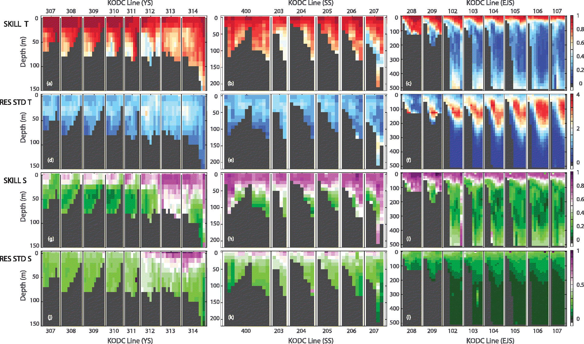
Fig. D1.
Zonal sections of the total skill (κ) and standard deviation () of the residual temperature (C) and salinity profiles sampled in the YS, SS, and EJS for a period of recent 20 years (1995 to 2014). (a–c) Total skill (κ) of the temperature. (d–f) Standard deviation () of the residual temperature. (g–i) Total skill (κ) of the salinity. (j–l) Standard deviation () of the residual salinity. (a), (d), (g), and (j): YS. (b), (e), (h), and (k): SS. (c), (f), (i), and (l): EJS. The vertical profiles are concatenated in terms of cross-shore lines, and the unsampled depths and bottom bathymetry are shown as gray columns.