
Table 1.
Gaussian approximations in DA algorithms.
[i] The “-” means “not applicable”. Smoothing algorithms can produce approximations of the filtering posterior by the smoother ensemble and the numerical model. The resulting representation of the filtering posterior is not Gaussian. For that reason, smoothing algorithms do not utilize Gaussian approximations of the filtering posterior. Whether or not 4D-Var makes a Gaussian approximation of the smoothing posterior depends on its implementation (see text for more detail).
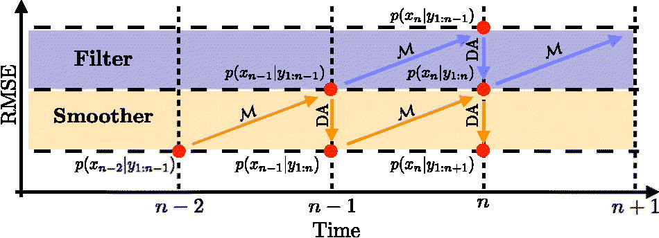
Fig. 1. A simplified schematic diagram of the RMSE of filters and smoothers. Diagonal arrows represent the model and vertical (downward) arrows represent assimilation of observations. The purple and orange regions illustrate the RMSE that the filter and smoother produce.
Table 2.
Filtering prior, filtering posterior and smoothing posterior of two nonlinear examples.
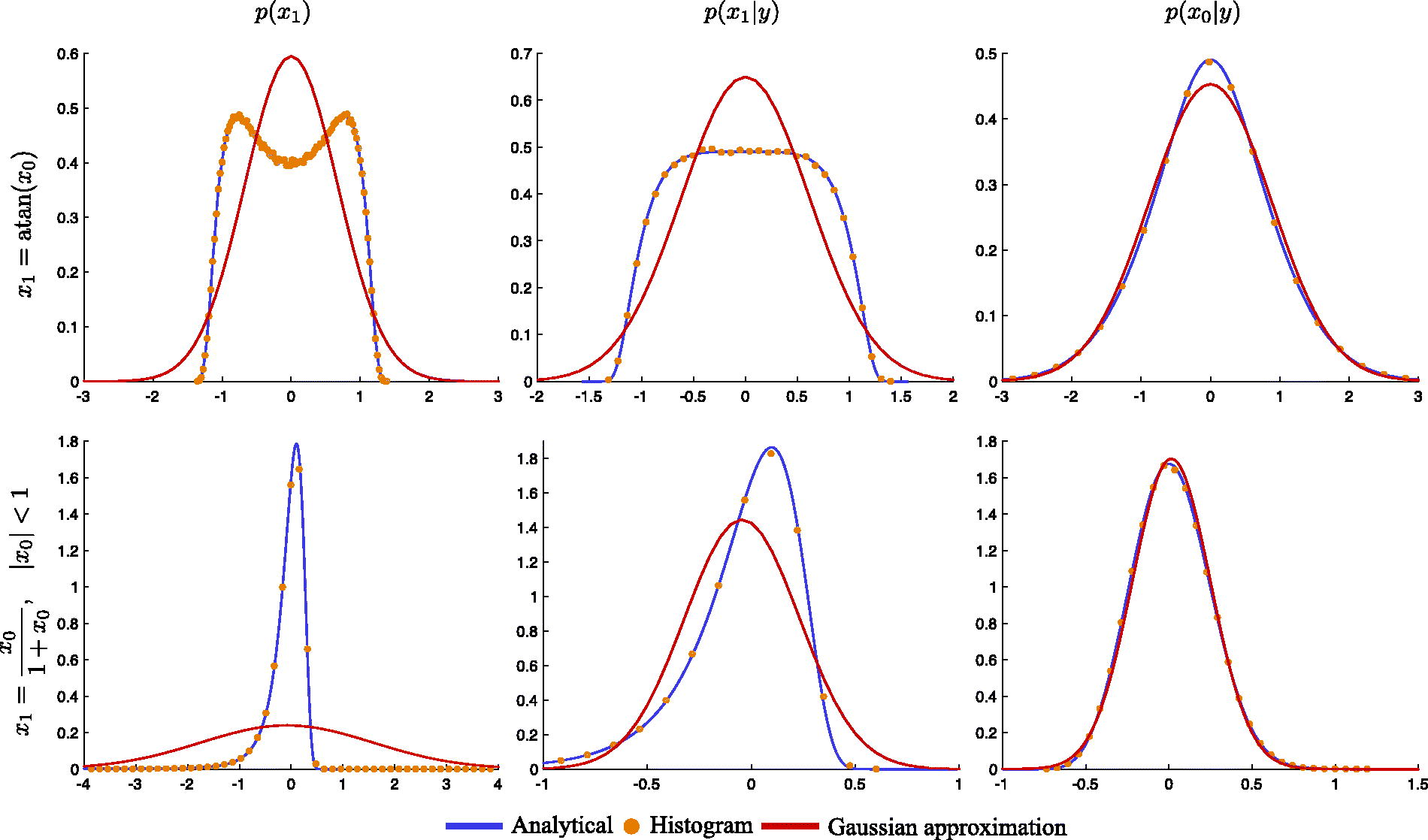
Fig. 2.
Filtering prior (left), filtering posterior (center) and smoothing posterior (right) of two nonlinear models. Top row: Bottom row: Shown are the distributions in blue, the bin heights of histograms obtained from 106 samples as orange dots, and a Gaussian approximation in red.
Table 3.
Skewness and excess kurtosis of filtering prior, filtering posterior and smoothing posterior of four nonlinear examples.
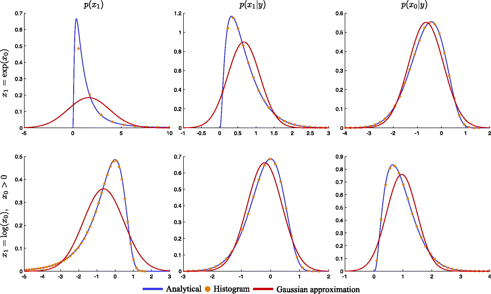
Fig. 3.
Filtering prior (left), filtering posterior (center) and smoothing posterior (right) of two nonlinear models. Top row: Bottom row: Shown are the distributions in blue, the bin heights of histograms obtained from 106 samples as orange dots, and a Gaussian approximation in red.
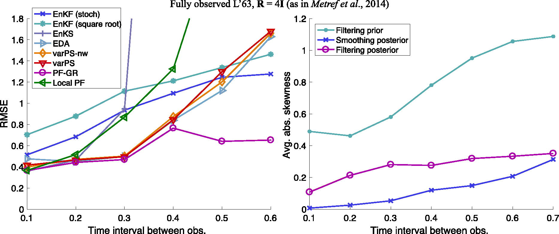
Fig. 4.
Left: RMSE as a function of the time interval between observations for a fully observed L63 system. Right: average of absolute value of skewness of filtering/smoothing priors and filtering/smoothing posteriors.
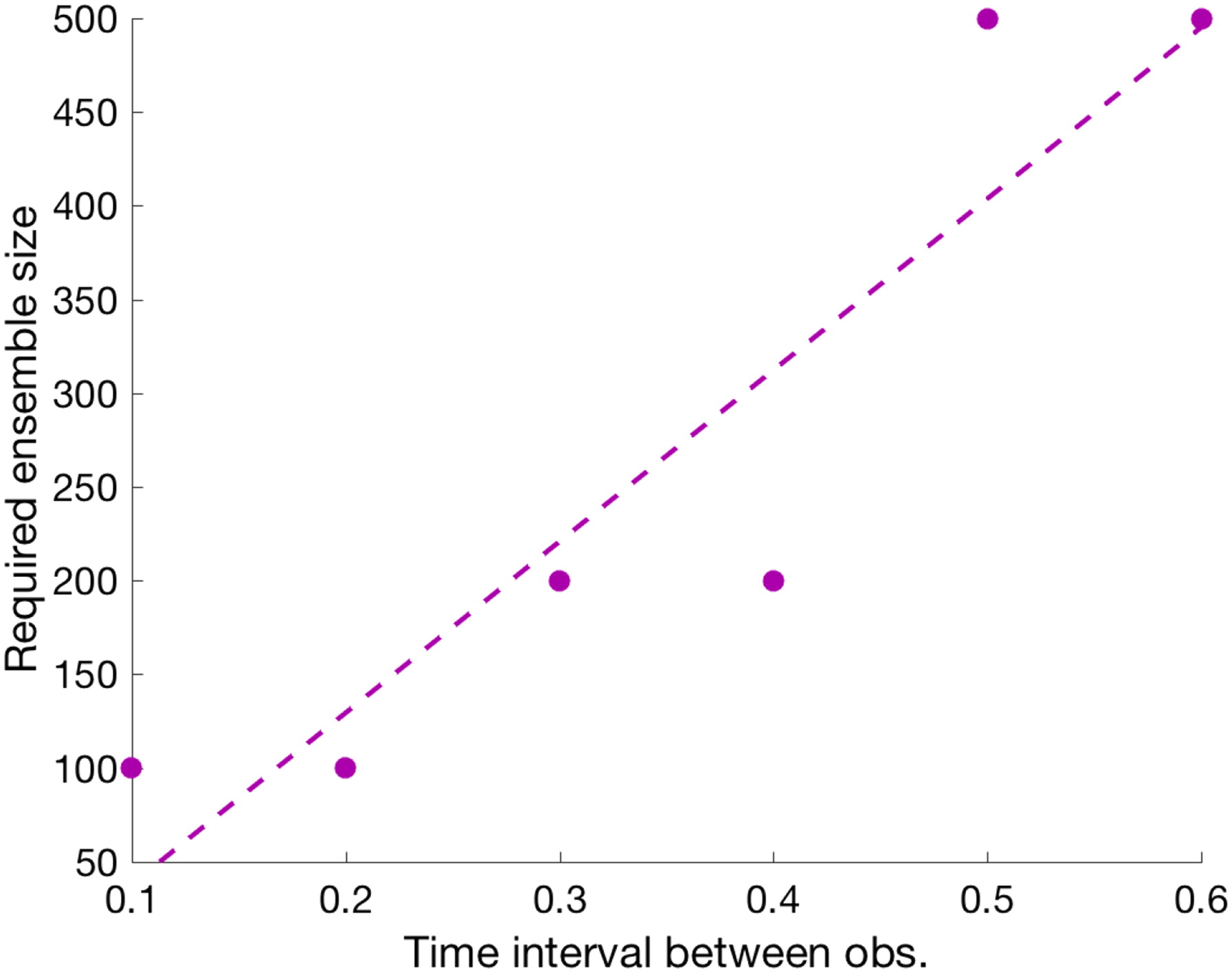
Fig. 5.
Ensemble size of the PF-GR required to reach RMSE of the PF-GR with ensemble size as a function of the time interval between observations. The dots correspond to results we obtained by considering the ensemble sizes and the dashed line is a least squares fit.
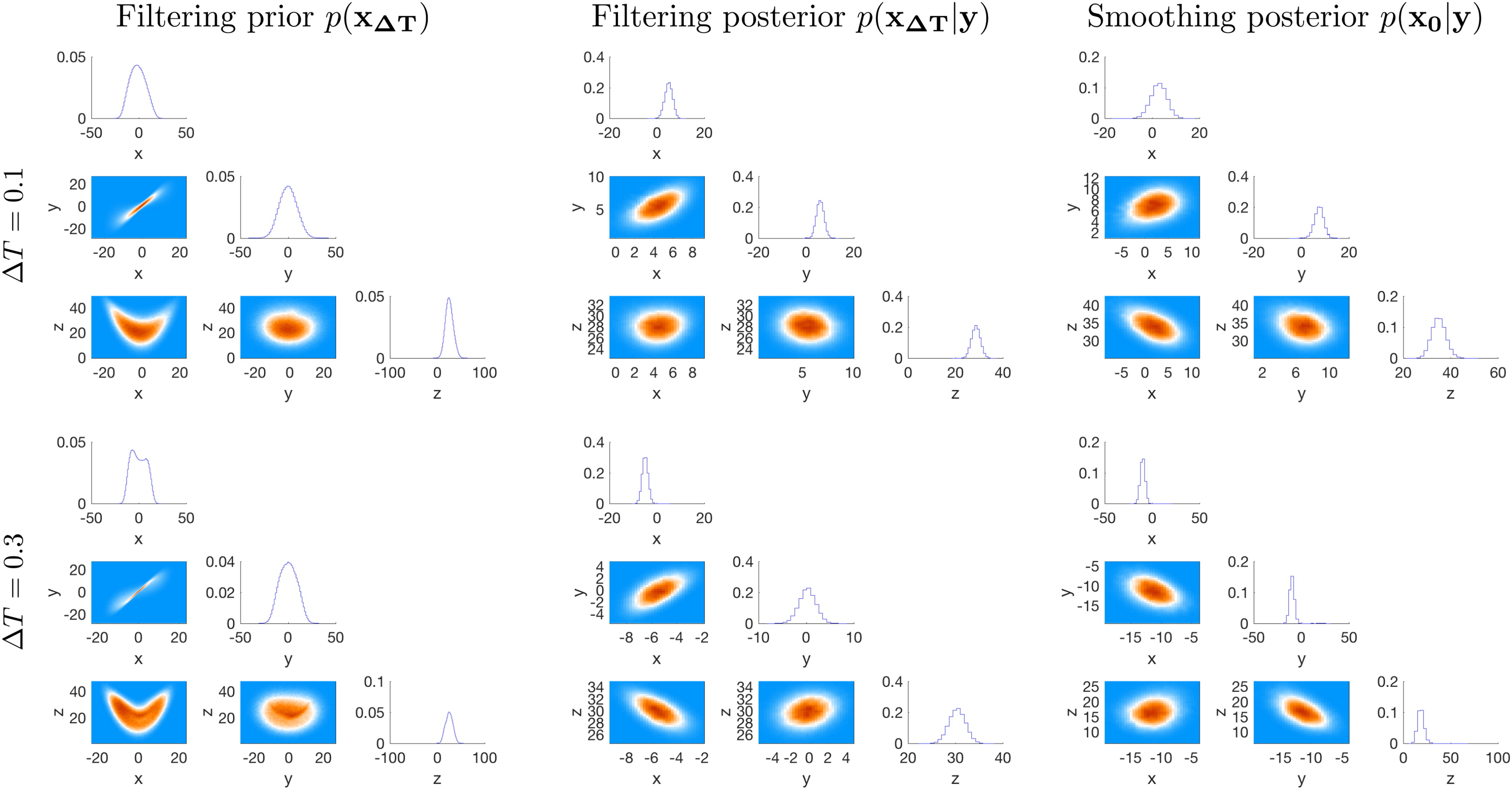
Fig. 6.
Corner plots of prior and posterior distributions for two different time intervals between observations.
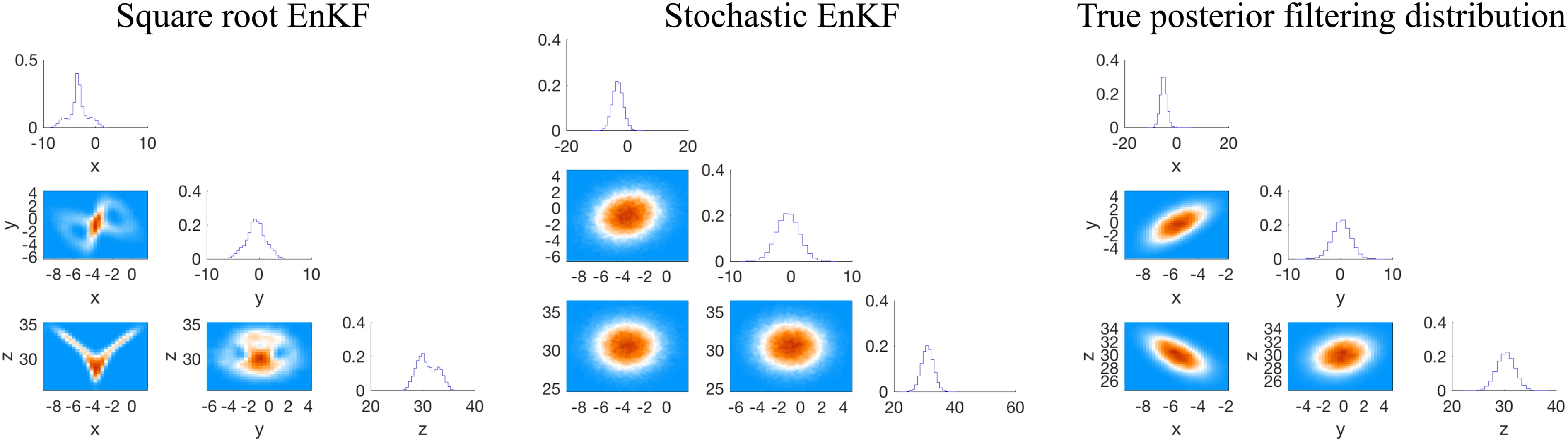
Fig. 7.
Corner plots of the analysis ensemble of of square root EnKF (left), stochastic EnKF (right). The time interval between observations is
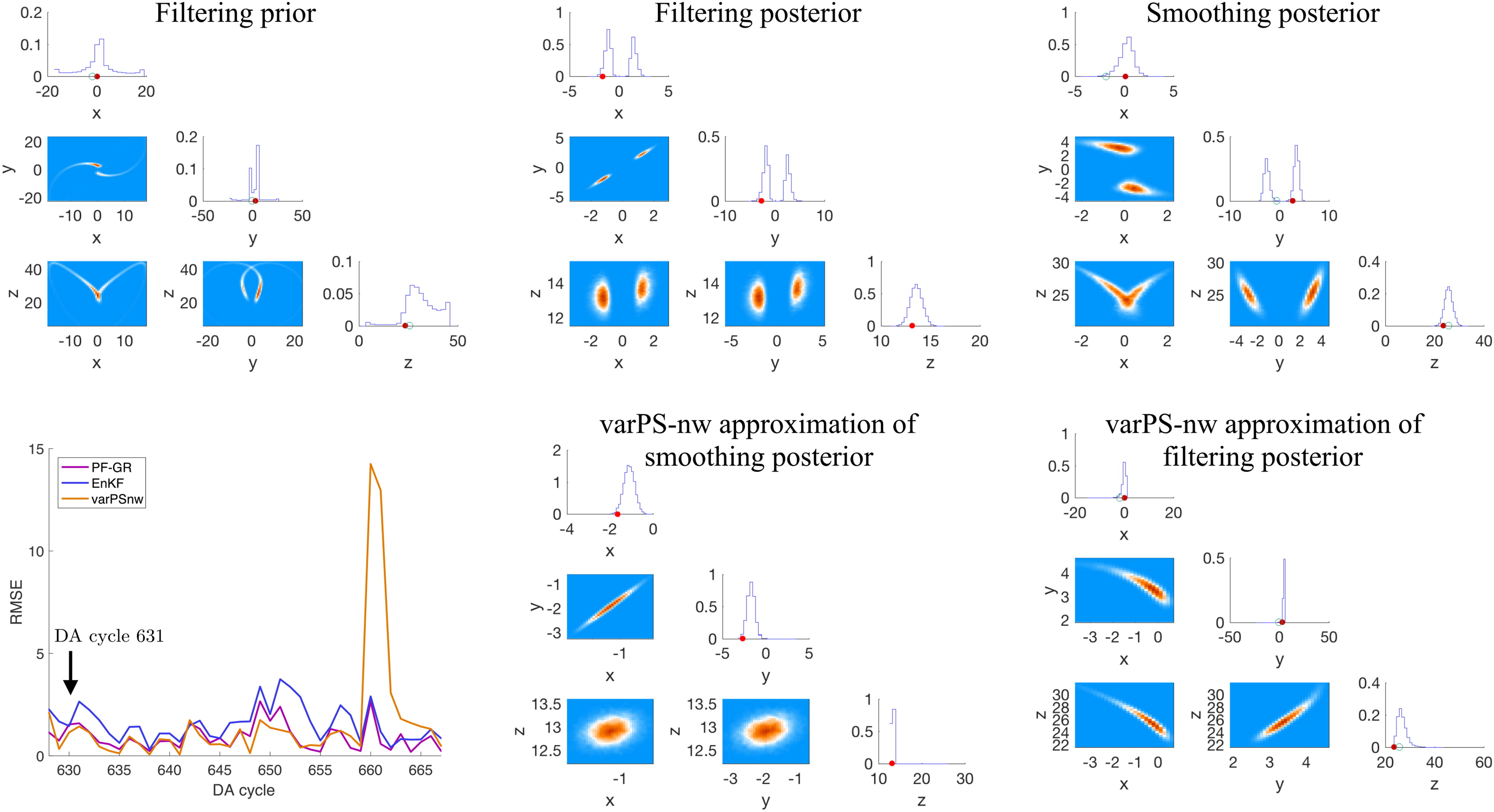
Fig. 8.
Top: corner plots of filtering prior (left), filtering posterior (center) and smoothing posterior (right) for DA cycle 631 with The histograms are obtained by running the PF-GR with The red dots are the true states and the orange dots are the observations. Bottom: RMSE as a function of DA cycle (left) and the varPS-nw approximations of the filtering posterior (center) and smoothing posterior (right).
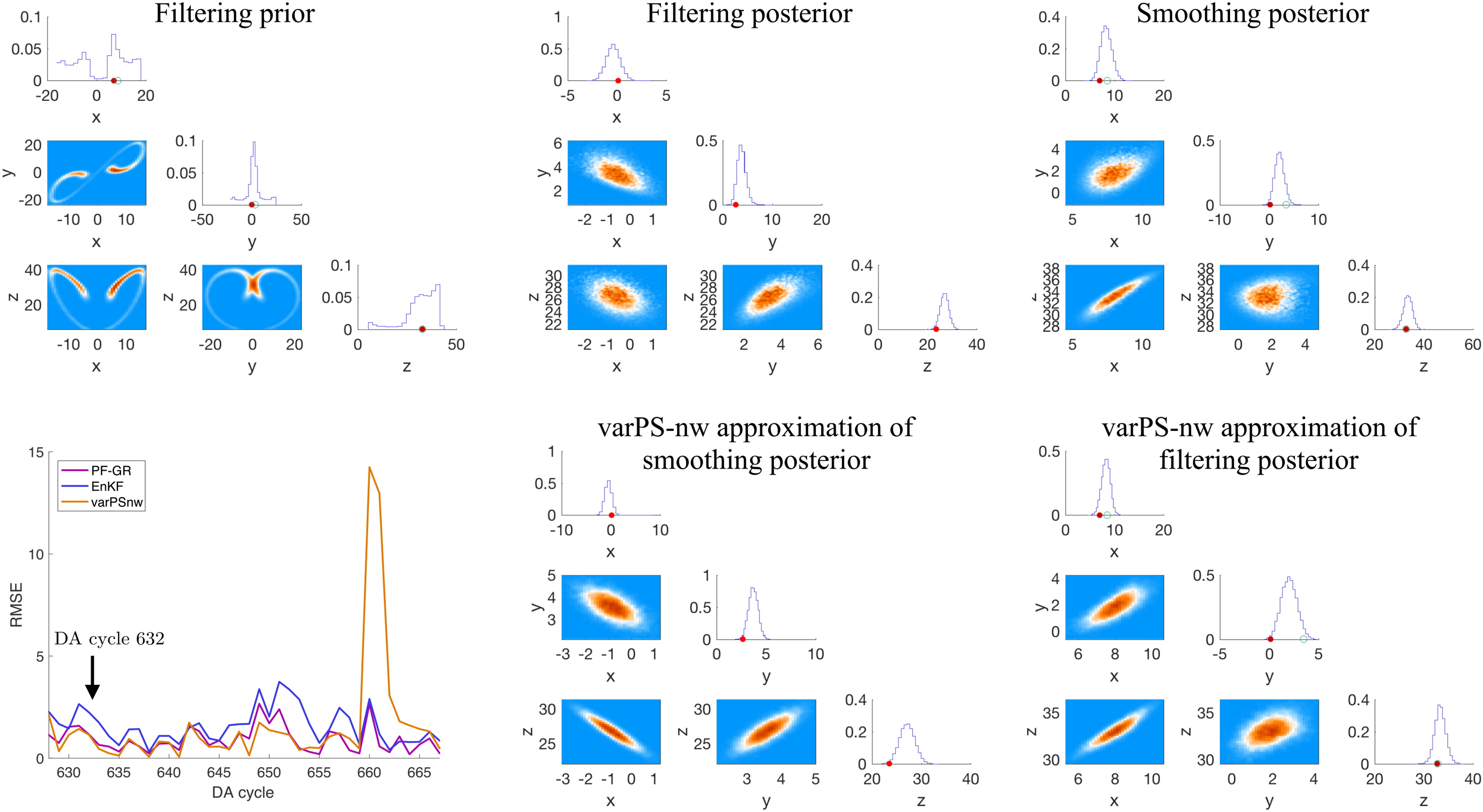
Fig. 9.
Top: corner plots of filtering prior (left), filtering posterior (center) and smoothing posterior (right) for DA cycle 632 with The histograms are obtained by running the PF-GR with The red dots are the true states and the orange dots are the observations. Bottom: RMSE as a function of DA cycle (left) and the varPS-nw approximations of the filtering posterior (center) and smoothing posterior (right).
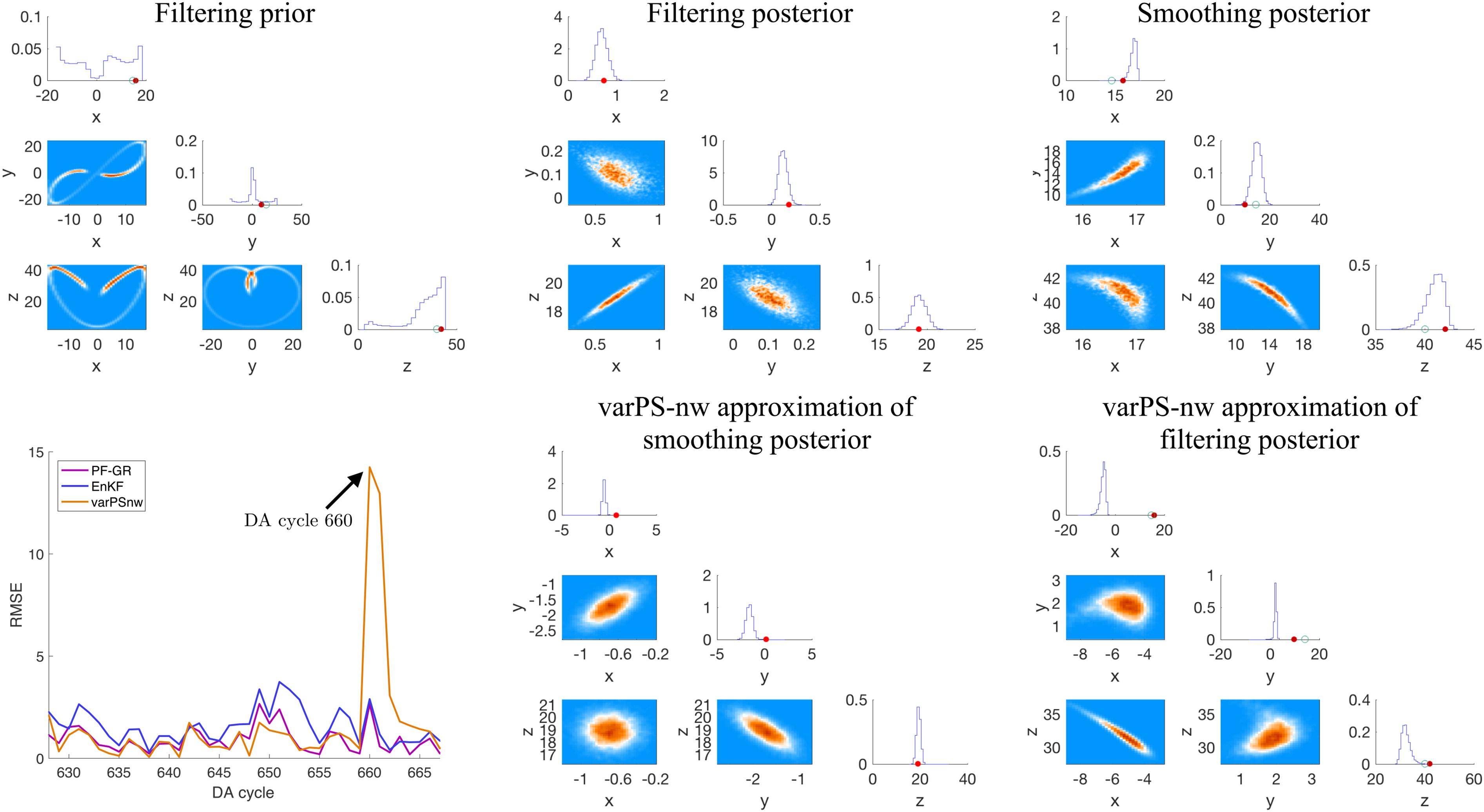
Fig. 10.
Top: corner plots of filtering prior (left), filtering posterior (center) and smoothing posterior (right) for DA cycle 660 with The histograms are obtained by running the PF-GR with The red dots are the true states and the orange dots are the observations. Bottom: RMSE as a function of DA cycle (left) and the varPS-nw approximations of the filtering posterior (center) and smoothing posterior (right).
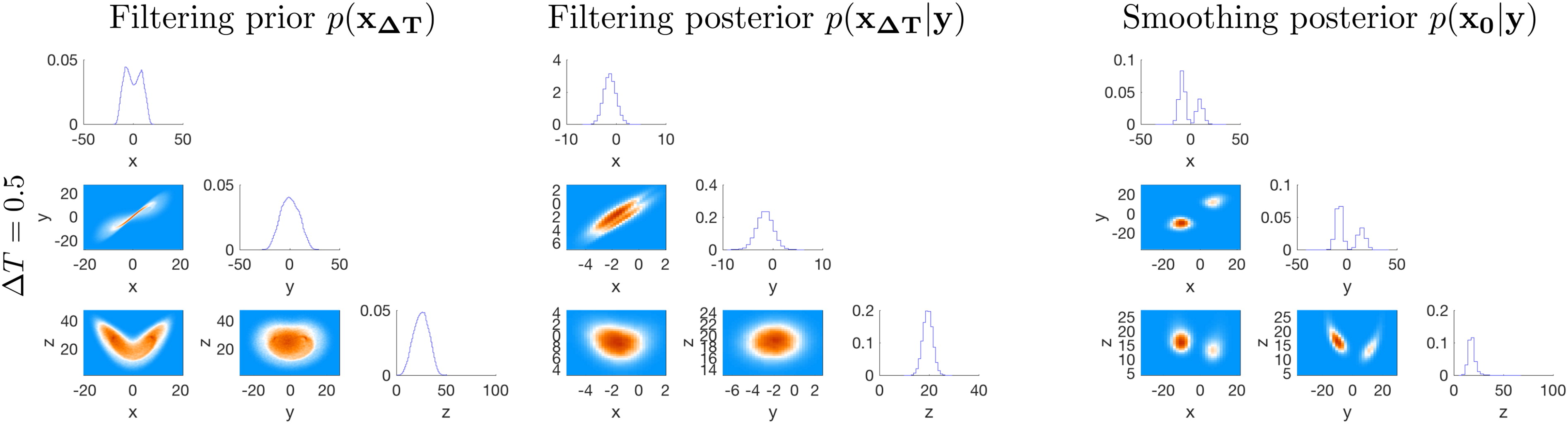
Fig. 11.
Corner plots of the filtering prior, filtering posterior and smoothing posterior distributions for a long time interval between observations ( strong nonlinearity).
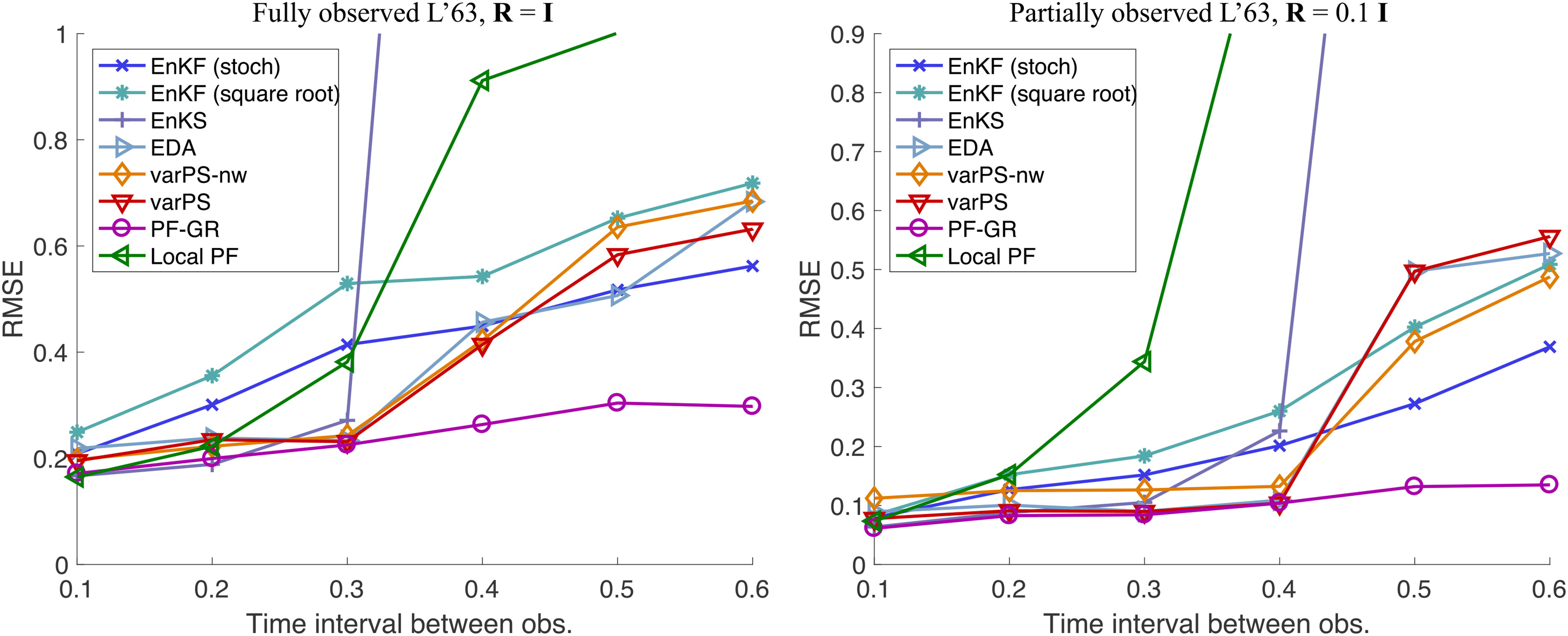
Fig. 12.
RMSE as a function of the time interval between observations for a fully observed L63 system (left) and a partially observed L63 system (right).
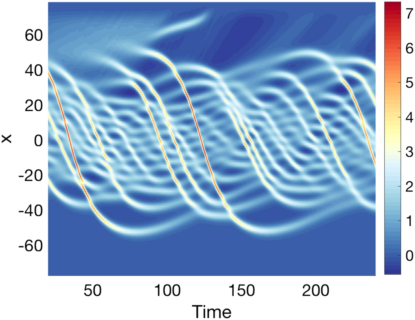
Fig. 13.
An example solution plotted in space and through time for the variable-coefficient KdV equation. The solitary waves are bouncing back-and-forth within a “potential well’ whose width is approximately defined between –40 and 40.
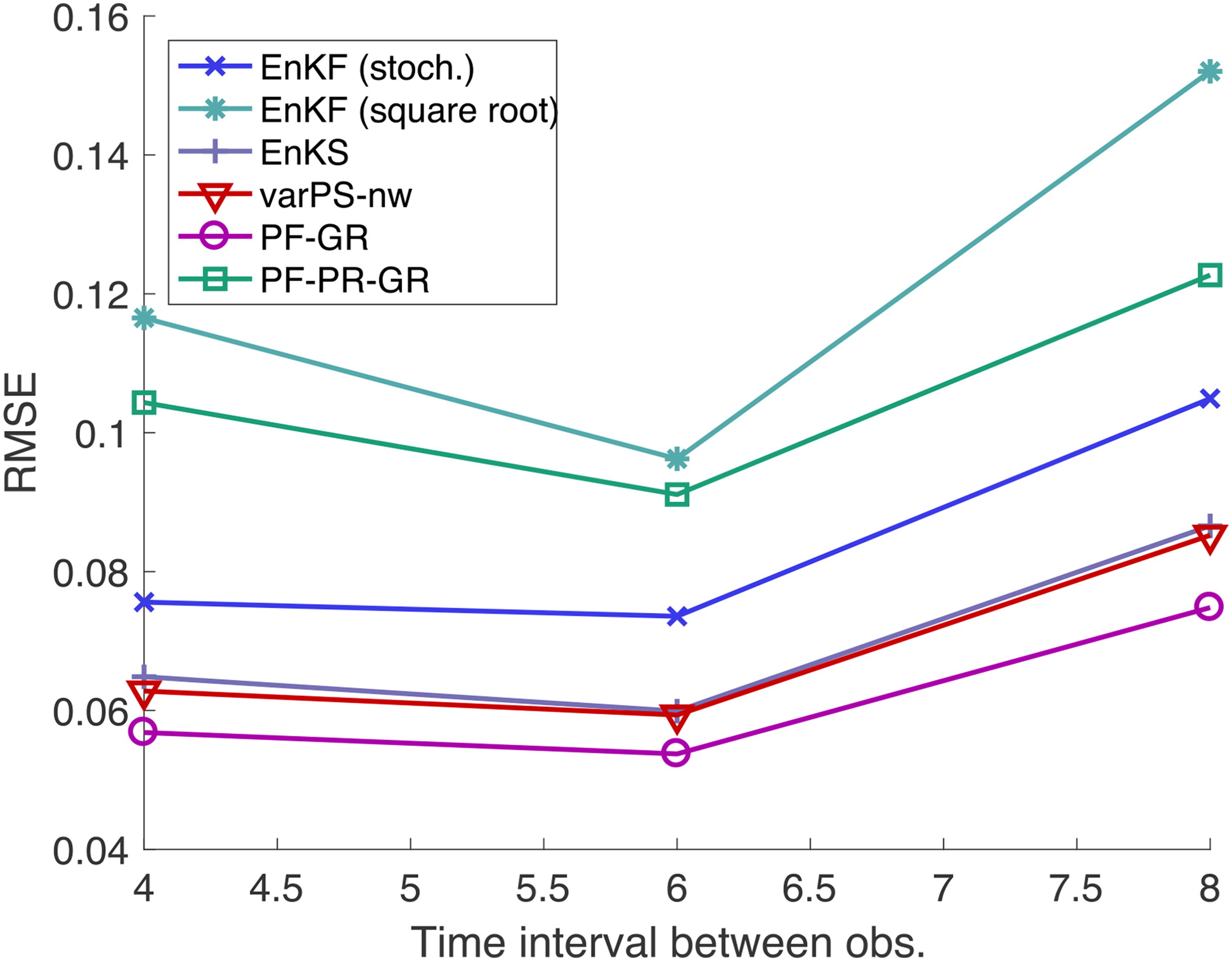
Fig. 14.
RMSE as a function of the time interval between observations for a partially observed KdV system.