
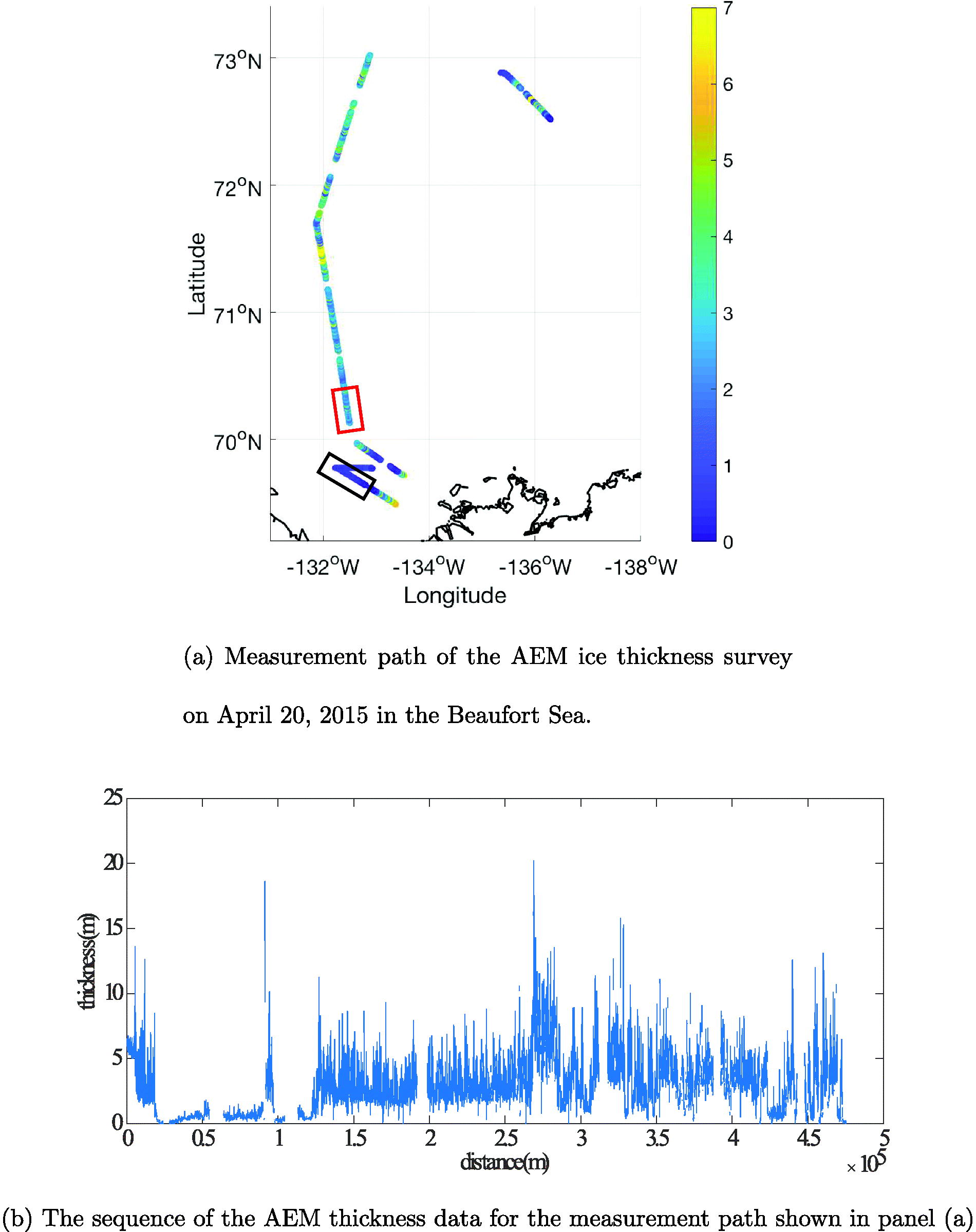
Fig. 1.
Sea ice thickness measurements from airborne electromagnetic (AEM) sensor in the Beaufort Sea acquired on 20 April 2015. (a) Sea ice thickness [m] is represented by the colorbar. The red rectangle outlines a region with deformed first year ice (FYI) while the black rectangle outlines a region with thinner and smoother first-year ice. These regions were determined from visual analysis of a SAR image acquired on 19 April 2015. (b) Sequential representation of the AEM data shown in panel (a).
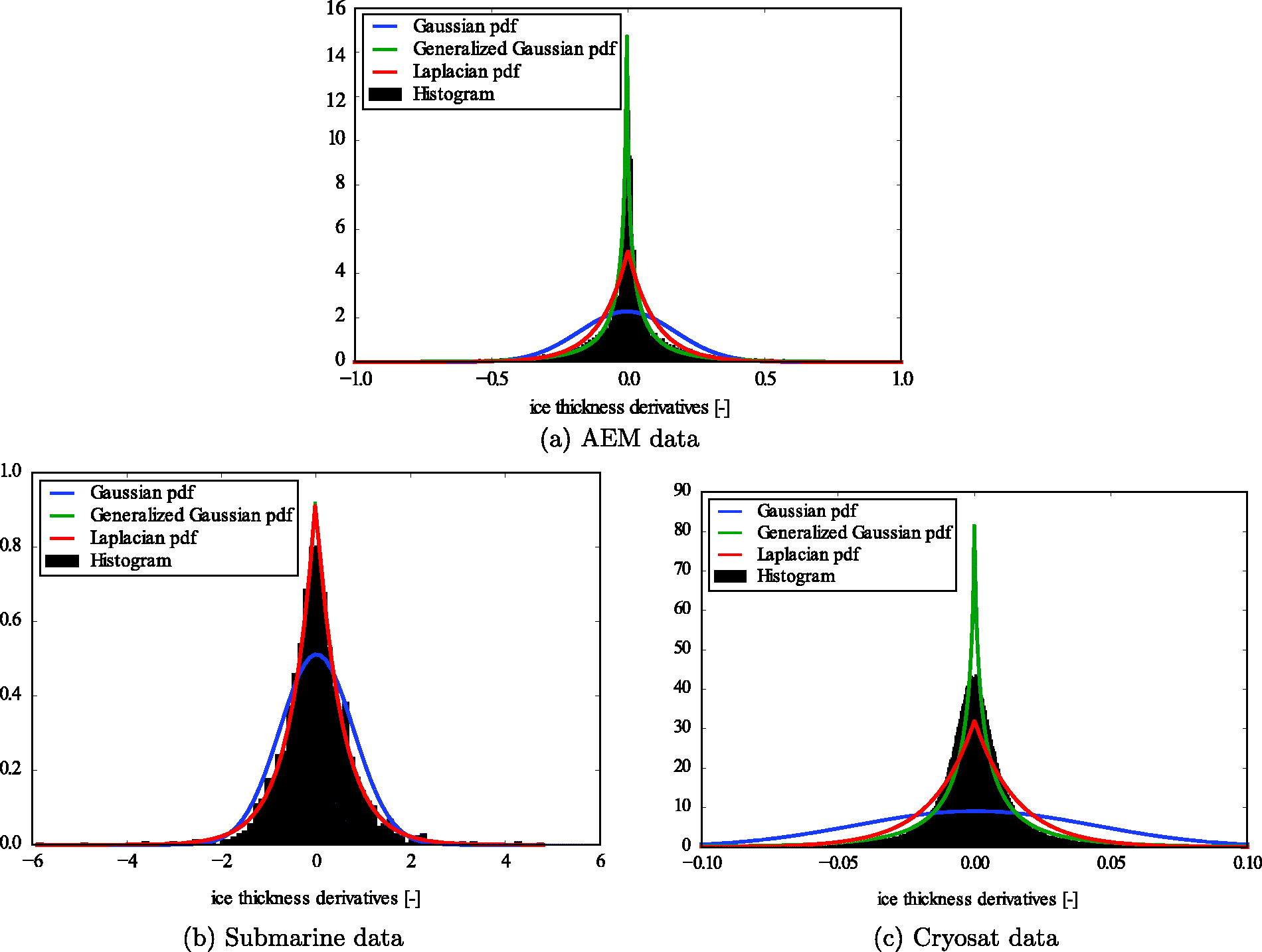
Fig. 2.
Normalised histograms of the ice thickness spatial derivative fields of AEM data (a), submarine data (b), and Cryosat data (c) with the fitted Gaussian, Laplacian and generalised Gaussian distributions. All histograms show more similarity to generalised Gaussian and Laplacian distributions rather than a Gaussian distribution. For the submarine data (b), the fitted generalised Gaussian distribution and the Laplacian distribution overlap.
Table 1.
Kullback-Leibler divergence (DKL) between different ice thickness datasets and their fitted distributions on the derivative field.
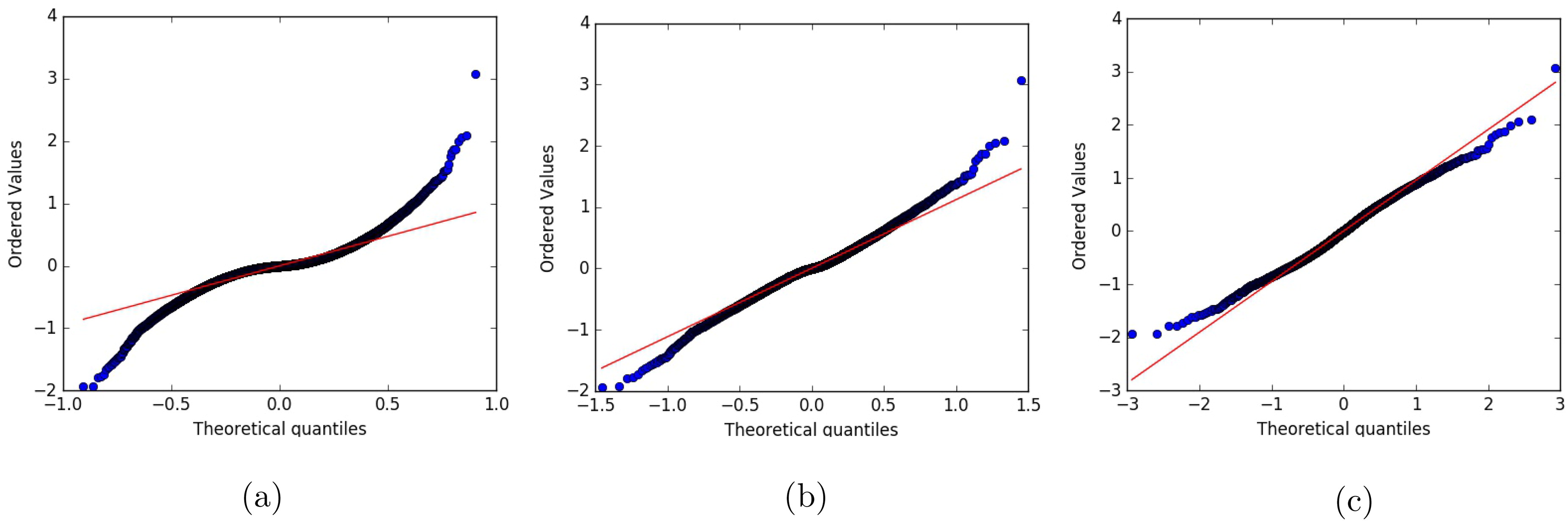
Fig. 3.
Q-Q plot of the data derivative field against Gaussian, Laplacian and generalised Gaussian distributions. The horizontal axes are the quantiles of the fitted distributions and the vertical axes are the ordered values of the derivative field of AEM data. Departure from the straight line indicates departure from the specified distribution. (a) Gaussian distribution; (b) Laplacian distribution; (c) Generalised Gaussian distribution.
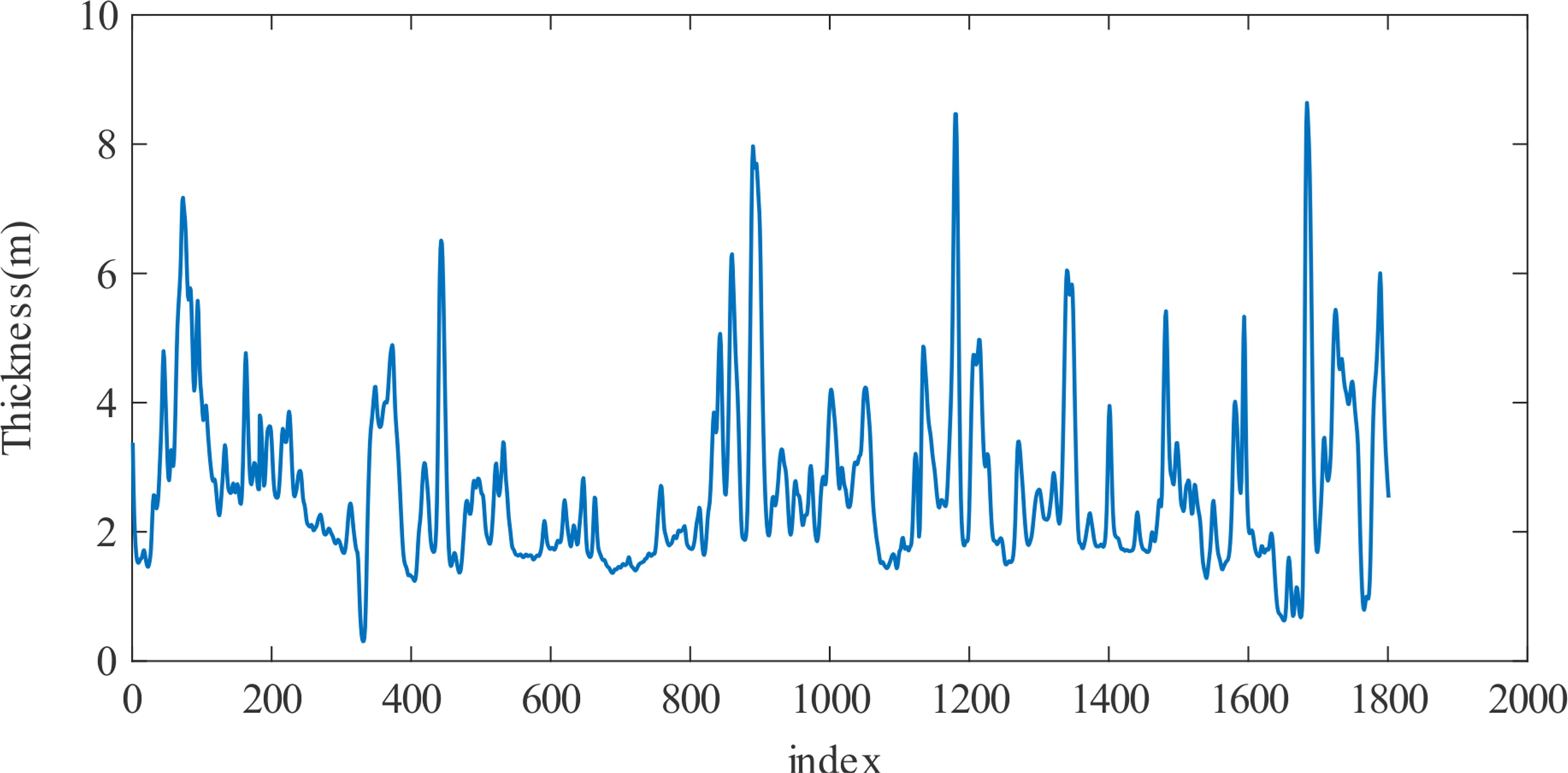
Fig. 4.
The deformed FYI sequence of the AEM thickness data outlined in Fig. 1 with red rectangle. The data points are spaced at 7 m.
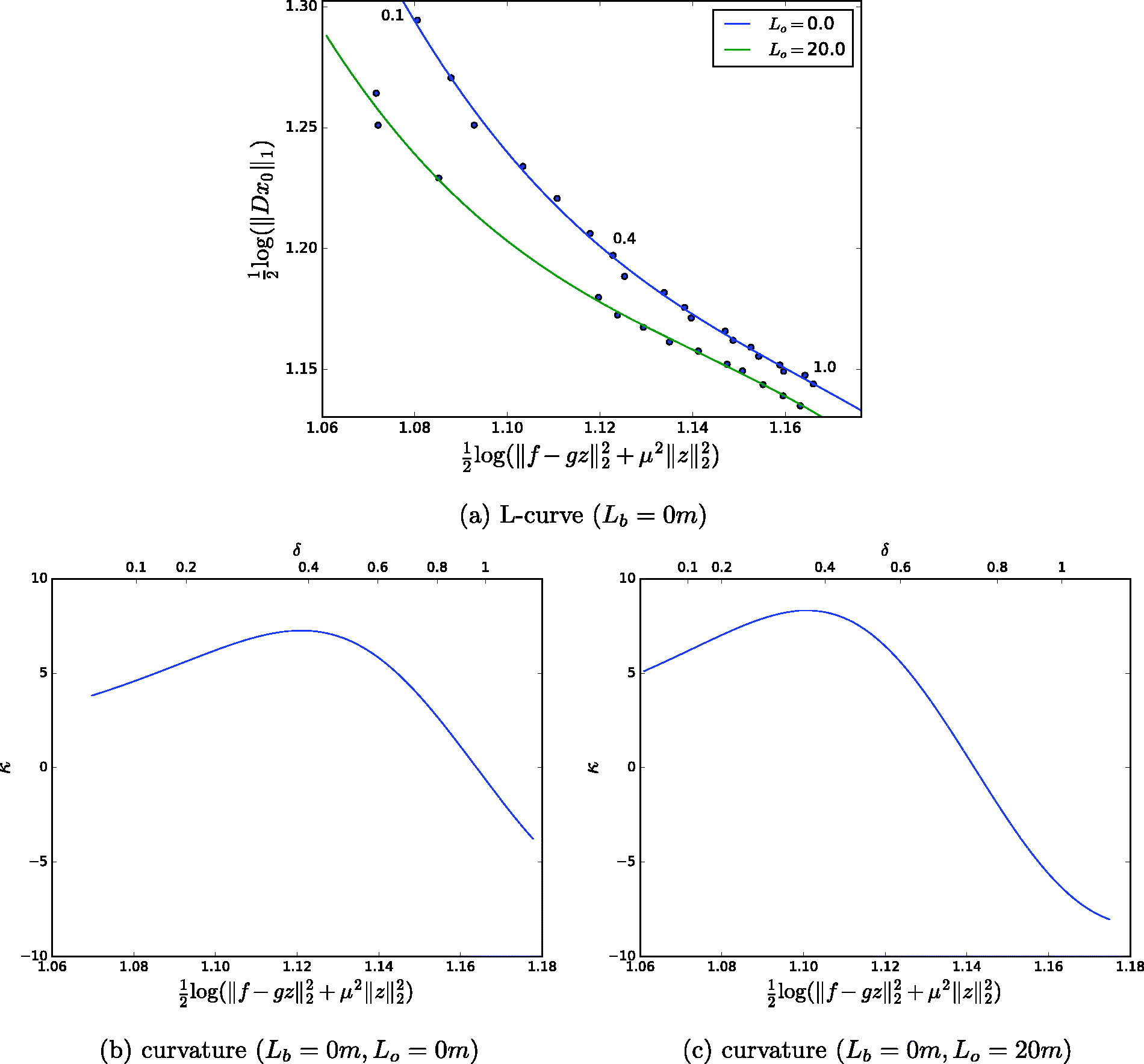
Fig. 5.
Using maximum curvature of L-curve to find regularisation parameter, δ. Panel (a) shows L-curve of two cases for which . In panel (b) and in panel (c) . The top axis of panels (b) and (c) shows the corresponding δ values for curvature points.
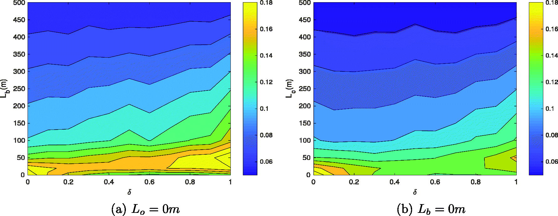
Fig. 6.
Analysis RMSE of the data fusion experiment over a range of δ values when (a) and Lb is changing and (b) and for a range of Lo values.
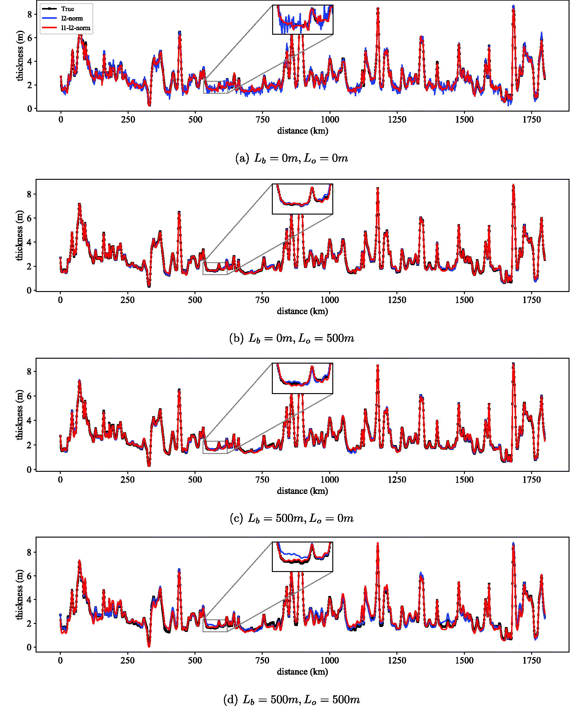
Fig. 7.
Data fusion analysis states for l2-norm (blue), l1–l2-norm (red) and true state (black) for different background and observation error correlation length scales for . (a) Lb = 0 m, Lo = 0 m; (b) Lb = 0 m, Lo = 500 m; (c) Lb = 500 m, Lo = 0 m; (d) Lb = 500 m, Lo = 500 m.
Table 2.
Data fusion analysis errors for different background and observation error correlation length scales (Lb and Lo) when and .
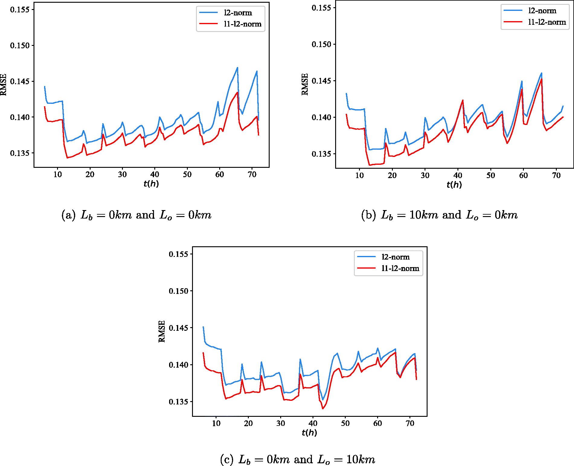
Fig. 8.
RMSE of the data assimilation ice thickness [m] states when (a) and , (b) and and (c) and for the 72 h data assimilation experiment. Data are assimilated every 6 h.
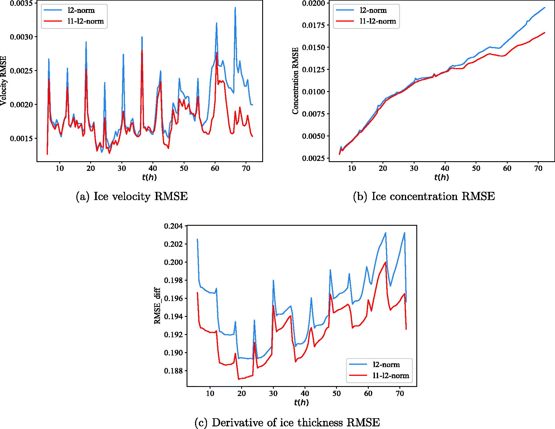
Fig. 9.
RMSE of the (a) ice velocity, (b) ice concentration and (c) ice thickness derivative when and for the 72 h data assimilation experiment. Data are assimilation every 6 h.
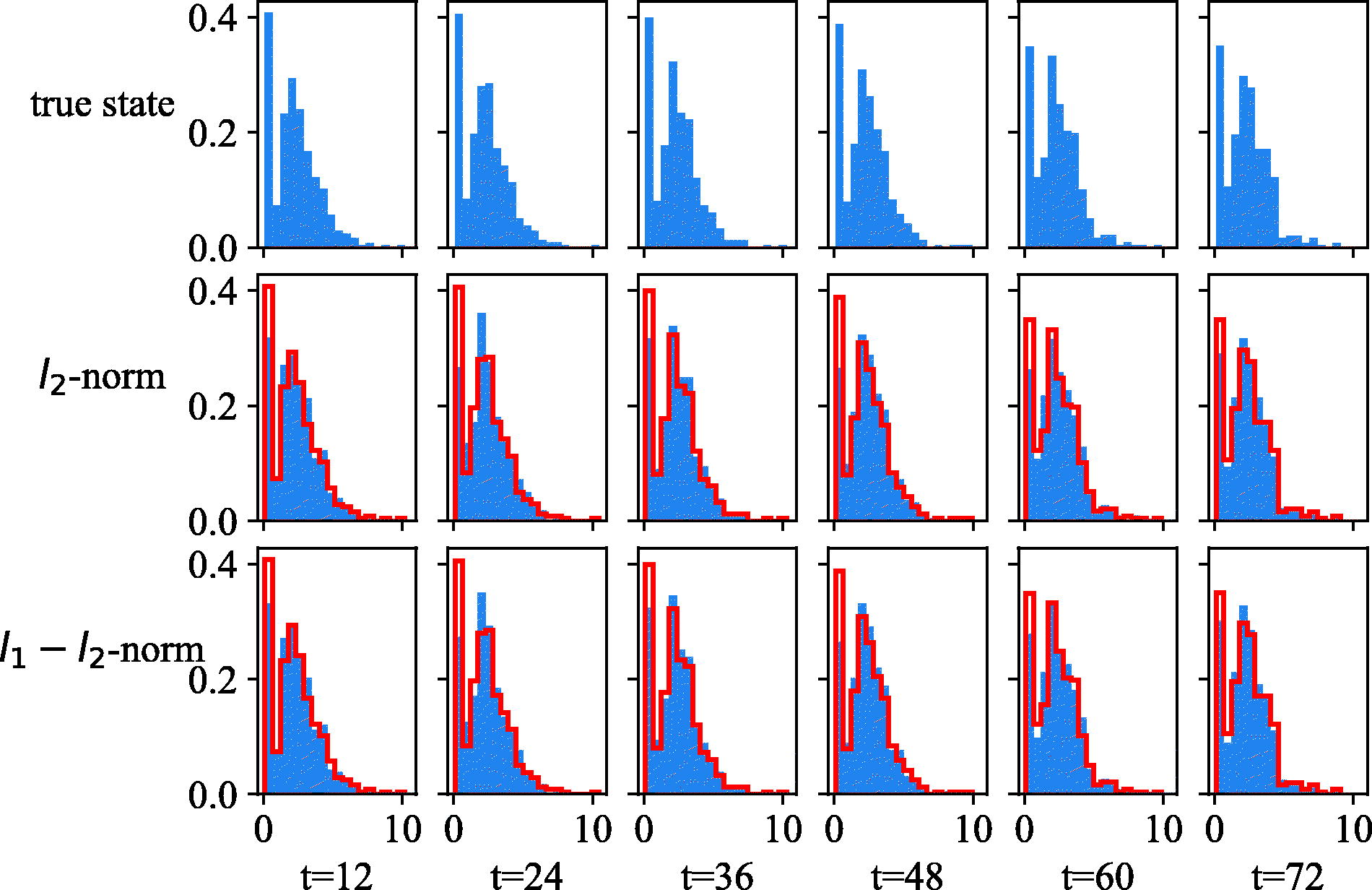
Fig. 10.
Histograms of the analysis states (ice thickness [m]) from the data assimilation when and . Each column shows the analysis state at the indicated time. The top row shows the true model, and the second and third rows show l2-norm and l1–l2-norm results, respectively. Histogram from the true state is overlayed by red colour in the second and third rows.
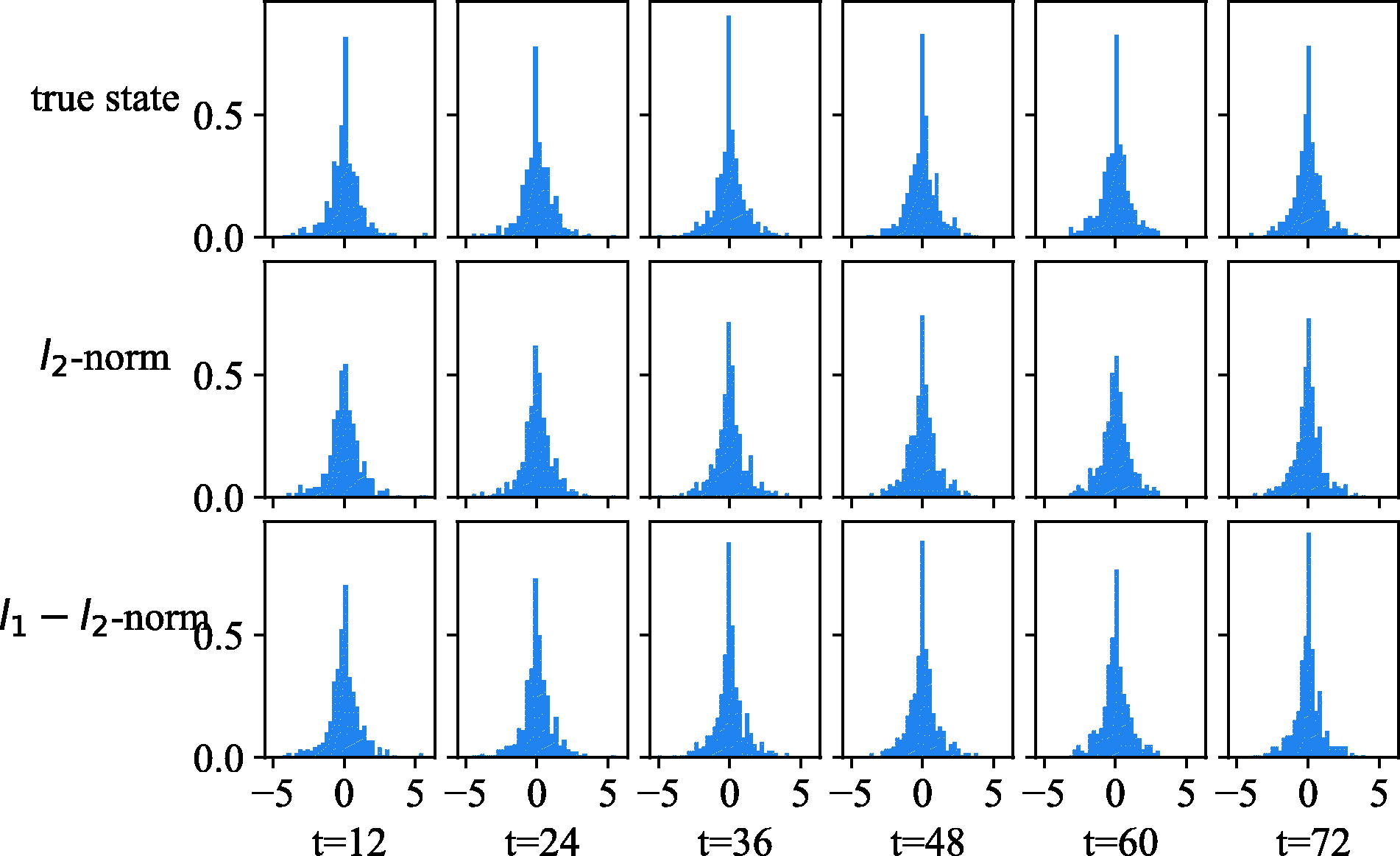
Fig. 11.
Histograms of the derivative of analysis states (ice thickness derivatives [−]) from data assimilation when and . Each column shows a different time step of the model. The top row shows the true model, and the second and third rows are showing l2-norm and l1–l2-norm results, respectively.
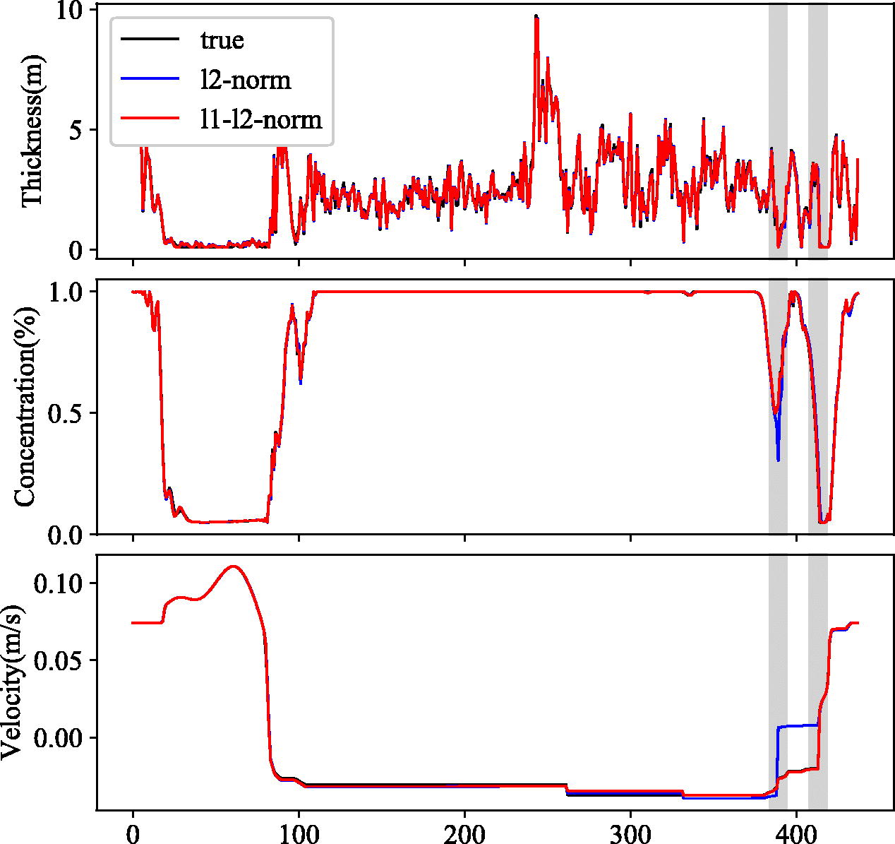
Fig. 12.
An example of data assimilation states at t = 64.0(h) when and . The shaded regions indicate the locations at which time traces (shown in Figs. 13 and 14) are taken.
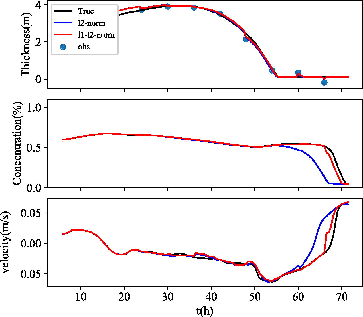
Fig. 13.
Model states from a single realisation of the data assimilation experiment for and at index = 389 (indicated by vertical line in Fig. 12). The decrease in ice concentration and thickness is overestimated for l2.
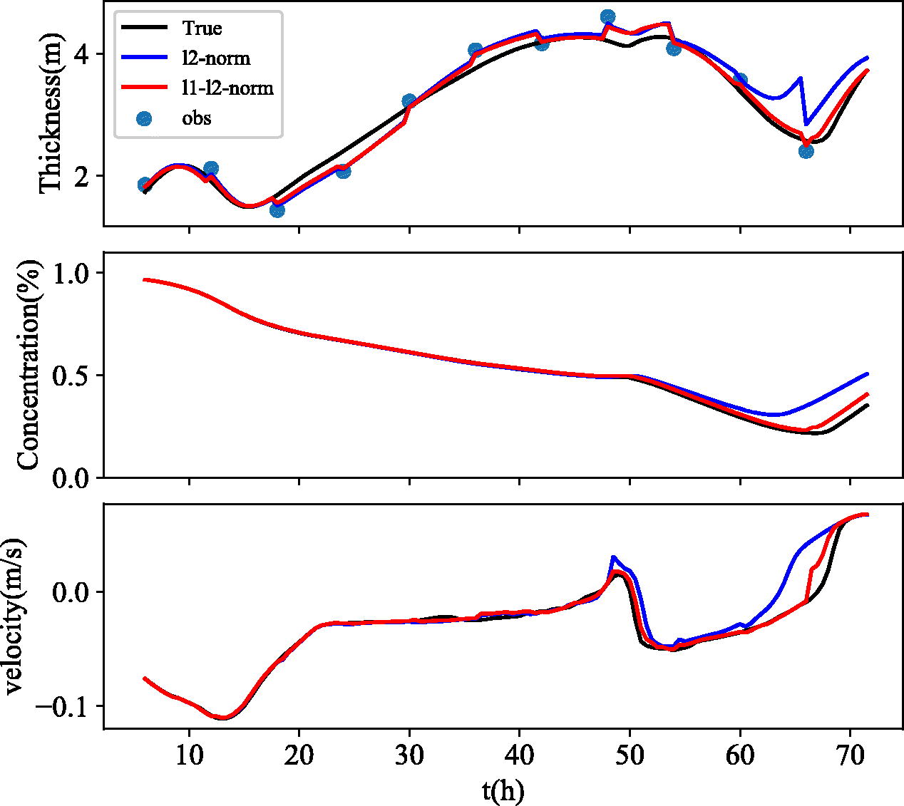
Fig. 14.
Model states from a single realisation of the data assimilation experiment for and at index = 245 (indicated by vertical line in Fig. 12). The opening in the ice cover is predicted better for the l1–l2 method than for the l2 method.