
Table 1.
Characteristics of ATMS window channels 16–17 and MHS window channels 1–2 onboard the NOAA-19 satellite.
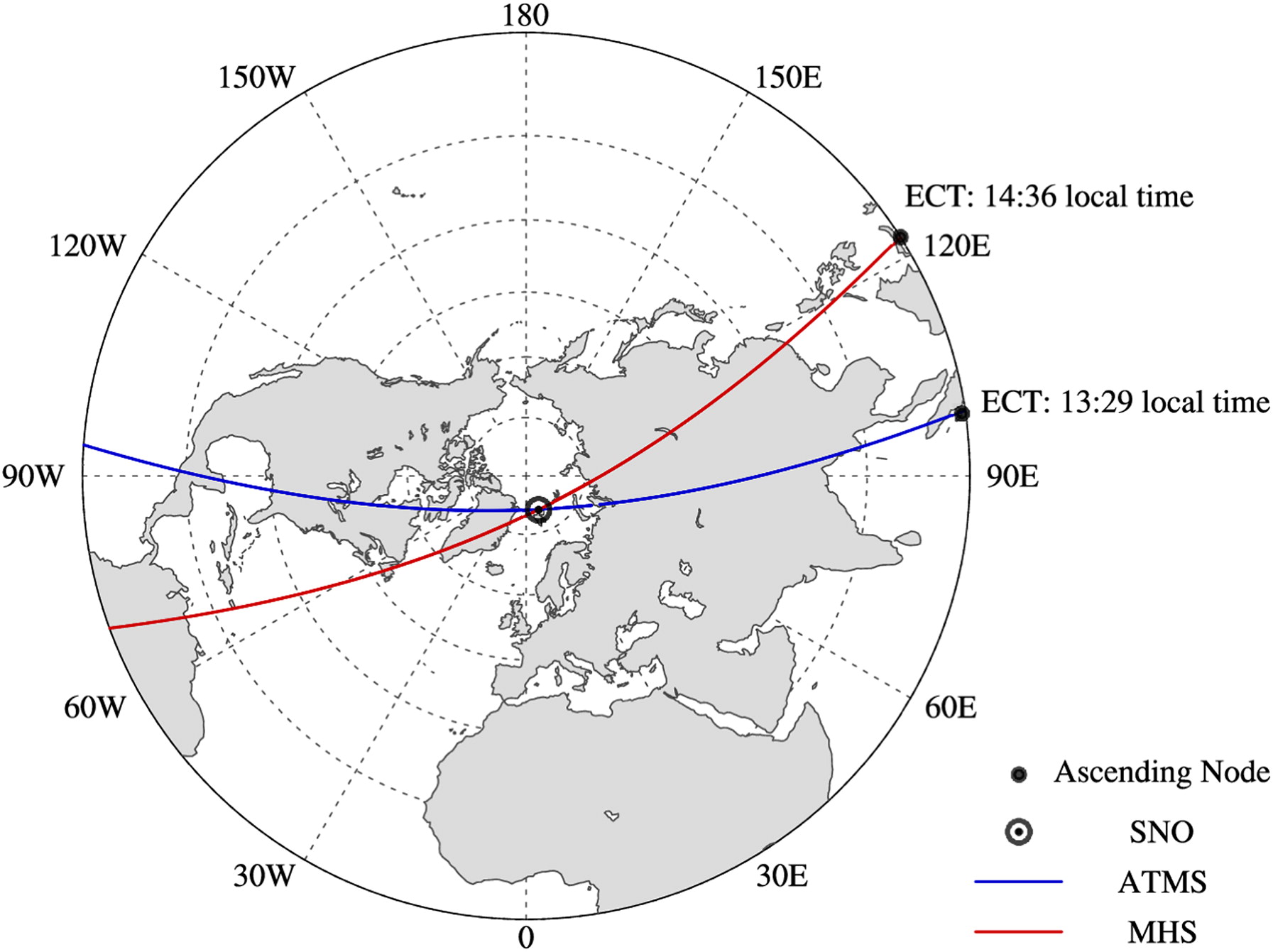
Fig. 1.
An ATMS and MHS simultaneous nadir overpass (SNO) point located at 20.1°E and 80.8°N and the associated ATMS (blue curve) and MHS (red curve) swaths on 8 January 2017 shown under a polar stereographic projection. The collocation criteria are 3 min in time and 8 km in spatial separation. The local equator crossing times (ECTs) of these two ATMS and MHS swaths are 1329 local time (LT) and 1436 LT, respectively.
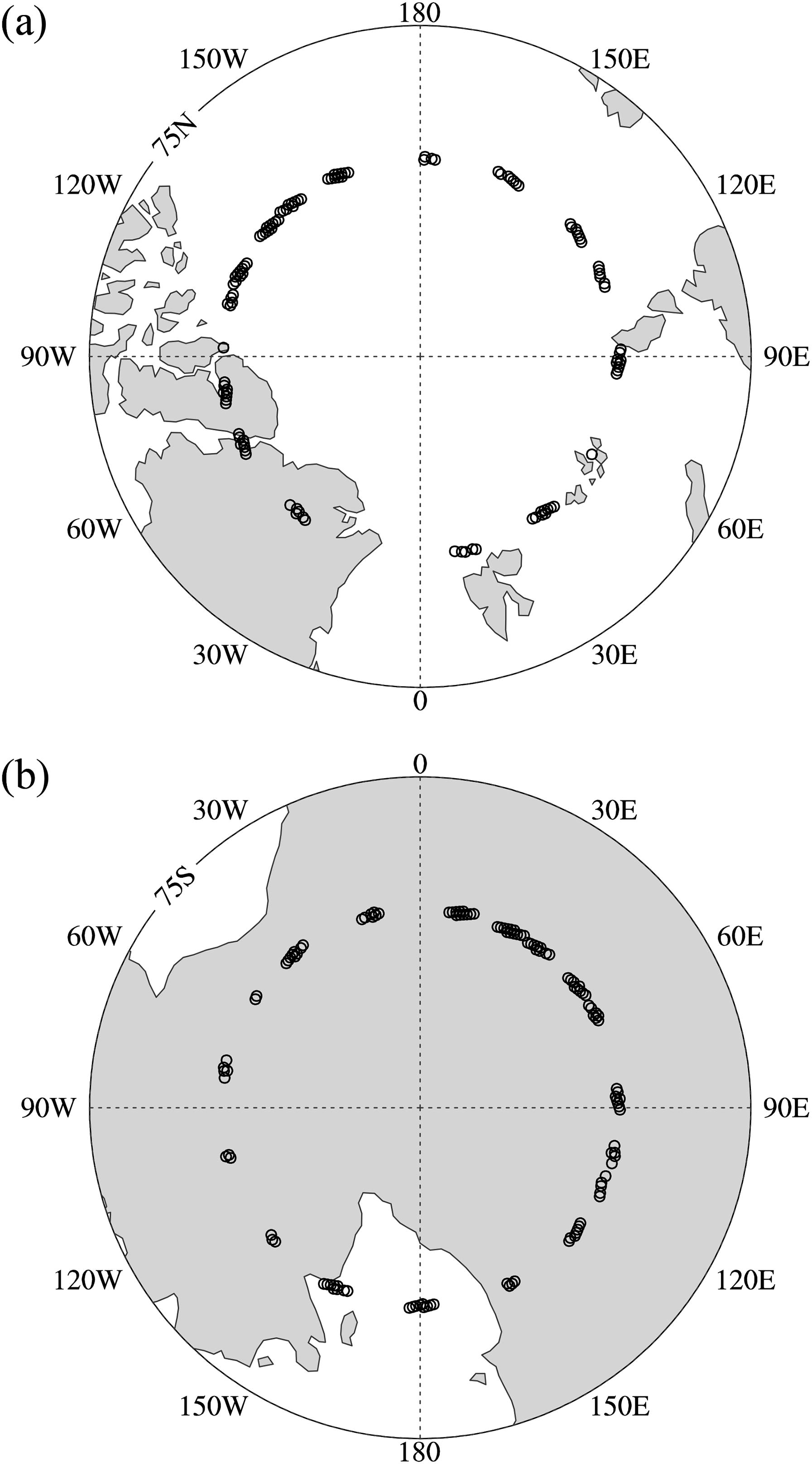
Fig. 2.
Geographical distributions of all SNOs found near the (a) North and (b) South Poles in January 2017 under a polar stereographic projection.
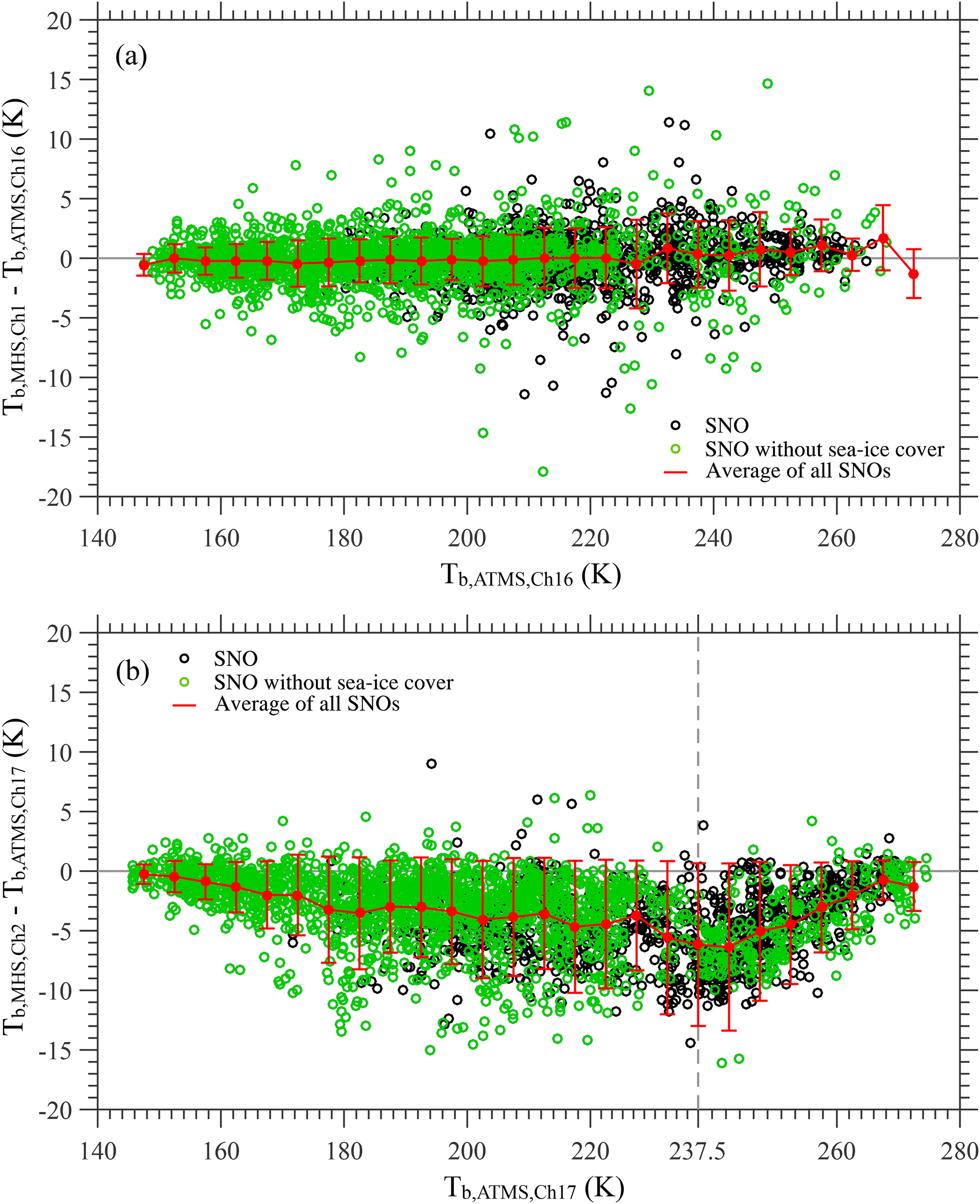
Fig. 3.
Scatterplots of the differences in observed brightness temperatures between (a) MHS channel 1 and ATMS channel 16, and (b) MHS channel 2 and ATMS channel 17 with respect to ATMS channel 16 and 17 observations without (green circles) and with (black circles) sea ice cover for a total of 3161 SNO points from May 2016 to April 2017. Means (solid red circles) and standard deviations (vertical red lines) are calculated at 5-K intervals. The dashed vertical line in (b) represents the pivot point demarking the decreasing and increasing trends (237.5 K).
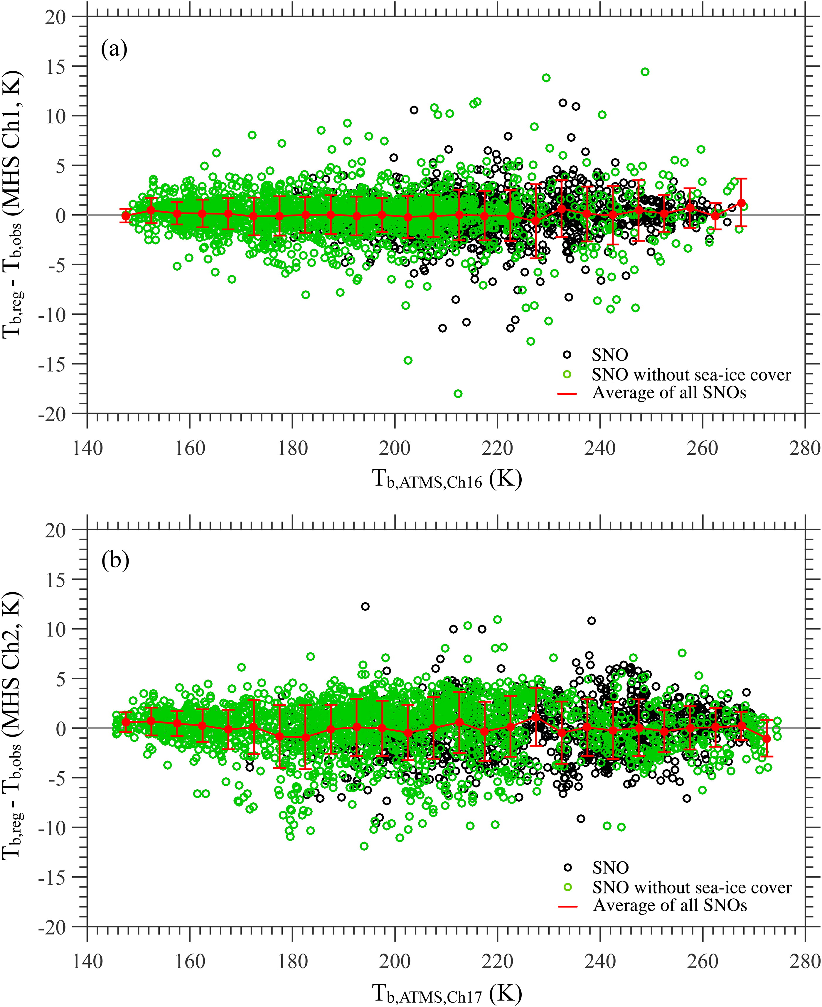
Fig. 4.
Same as Fig. 3 except for differences between regressed and observed MHS channel 1 (upper panel) and channel 2 (lower panel) brightness temperatures as a function of ATMS channel 16 and 17 brightness temperatures, respectively.
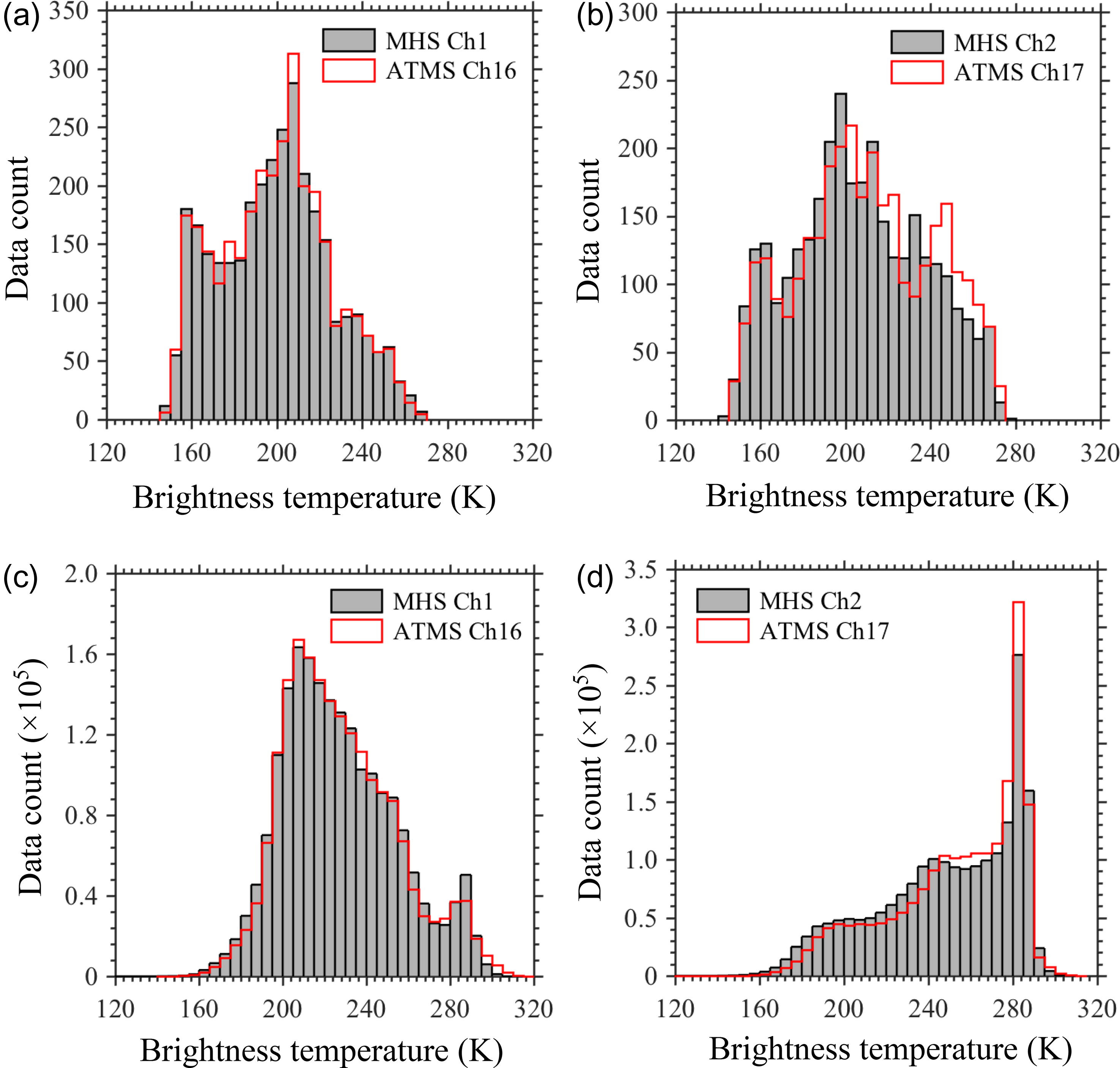
Fig. 5.
Histograms of brightness temperatures sampled by (a)–(b) the SNOs of the year from 1 May 2016 to 30 April 2017 and (c)-(d) one-month nadir measurements in January 2017.
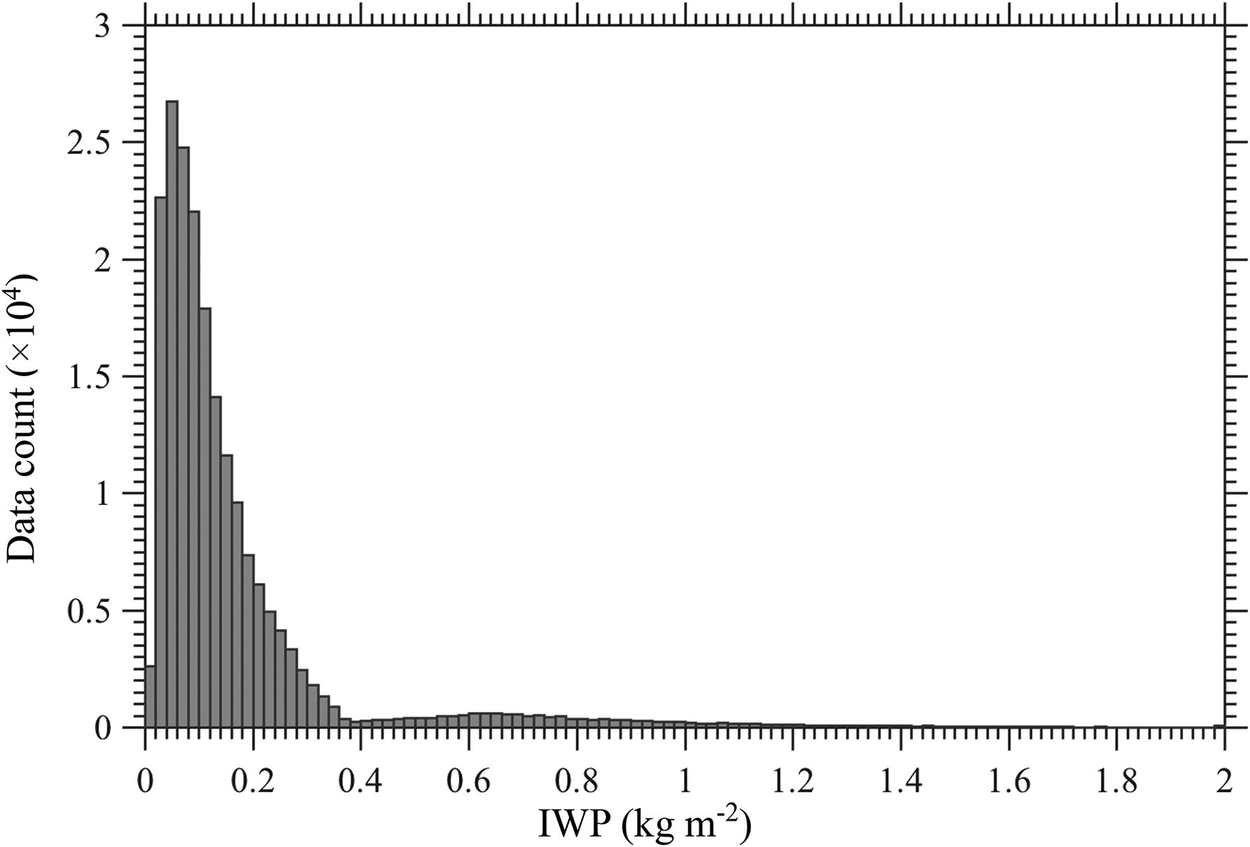
Fig. 6.
Data counts of MHS-retrieved IWP at 0.02 kg m−2 intervals calculated using the original MHS IWP retrieval algorithm for all data on 12 December 2016 and 4 February 2017.
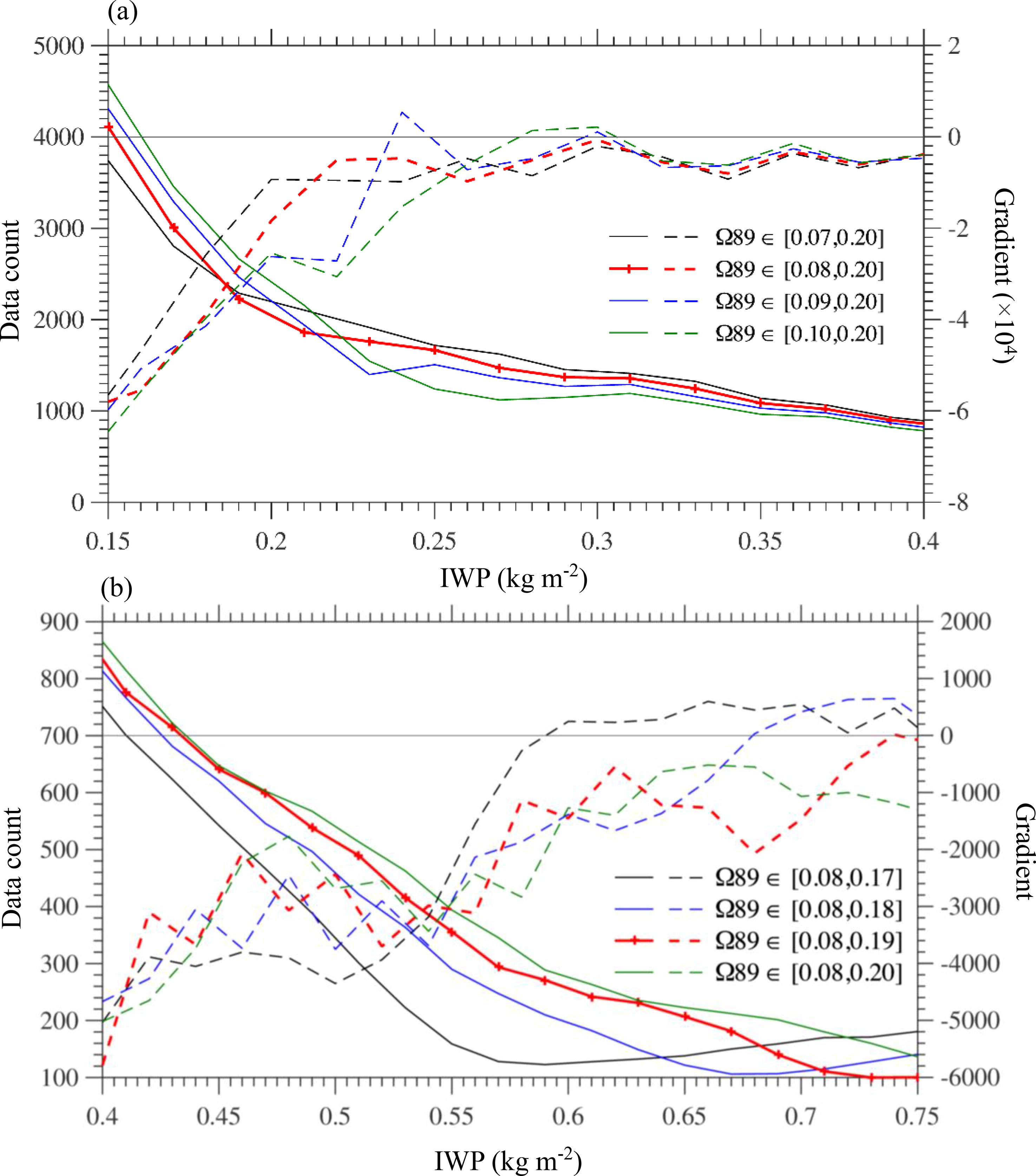
Fig. 7.
Variations in the data count with respect to the MHS-retrieved IWP at 0.02 kg m−2 intervals (solid curves) on 4 February 2017. The IWP retrieval scheme was applied for different ranges of Ω89: (a) 0.07–0.20 (black), 0.08–0.20 (red), 0.09–0.20 (blue), 0.10–0.20 (green), and (b) 0.08–0.17 (black), 0.08–0.18 (blue), 0.08–0.19 (red), and 0.08–0.20 (green). The gradients of the data counts are also shown (right-hand ordinate, dashed curves).
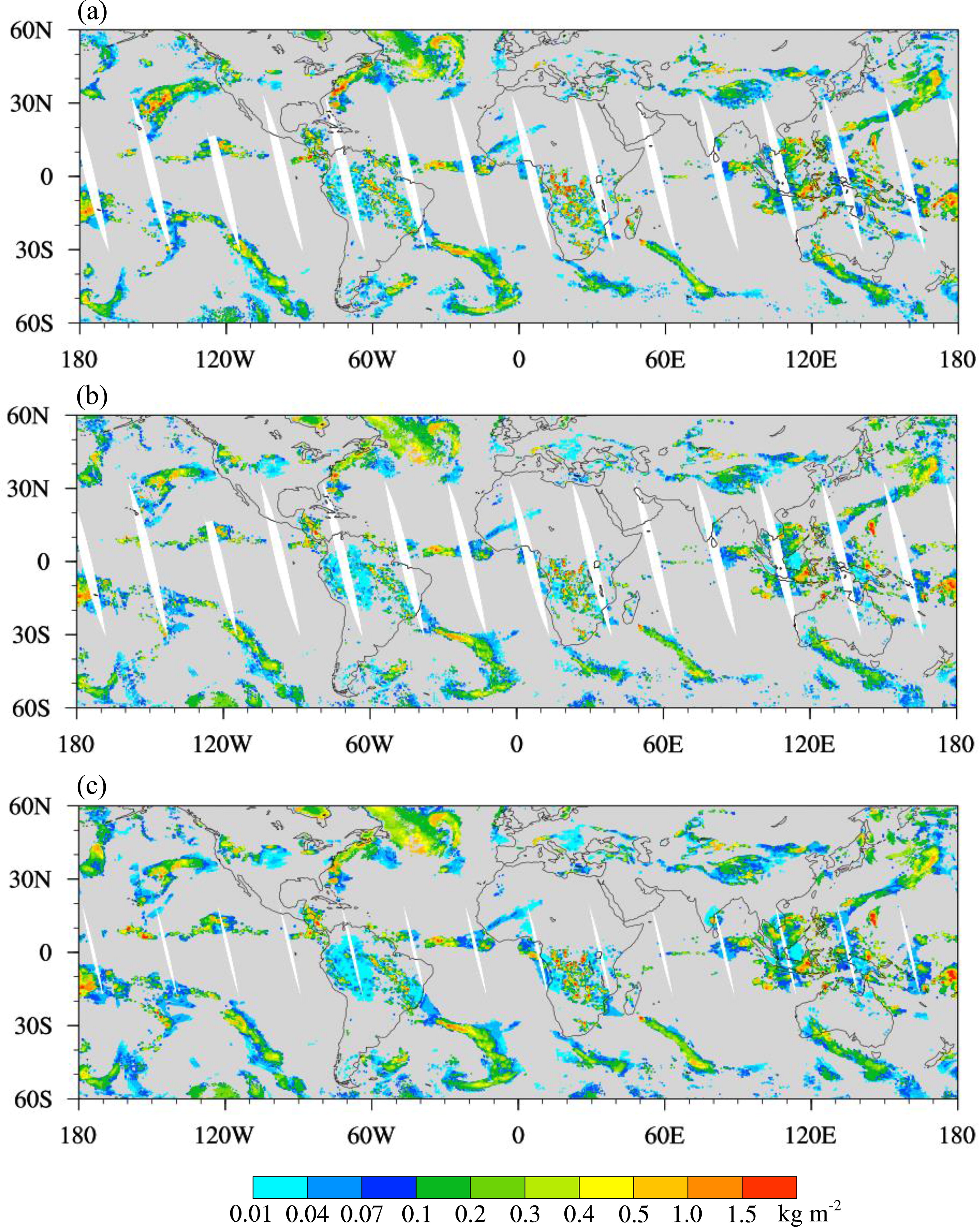
Fig. 8.
Spatial distributions of (a) MHS-retrieved IWP calculated by the modified algorithm, (b) ATMS-derived IWP overlaid on MHS swaths, and (c) ATMS-derived IWP calculated by the modified algorithm. Data are from 12 December 2016.
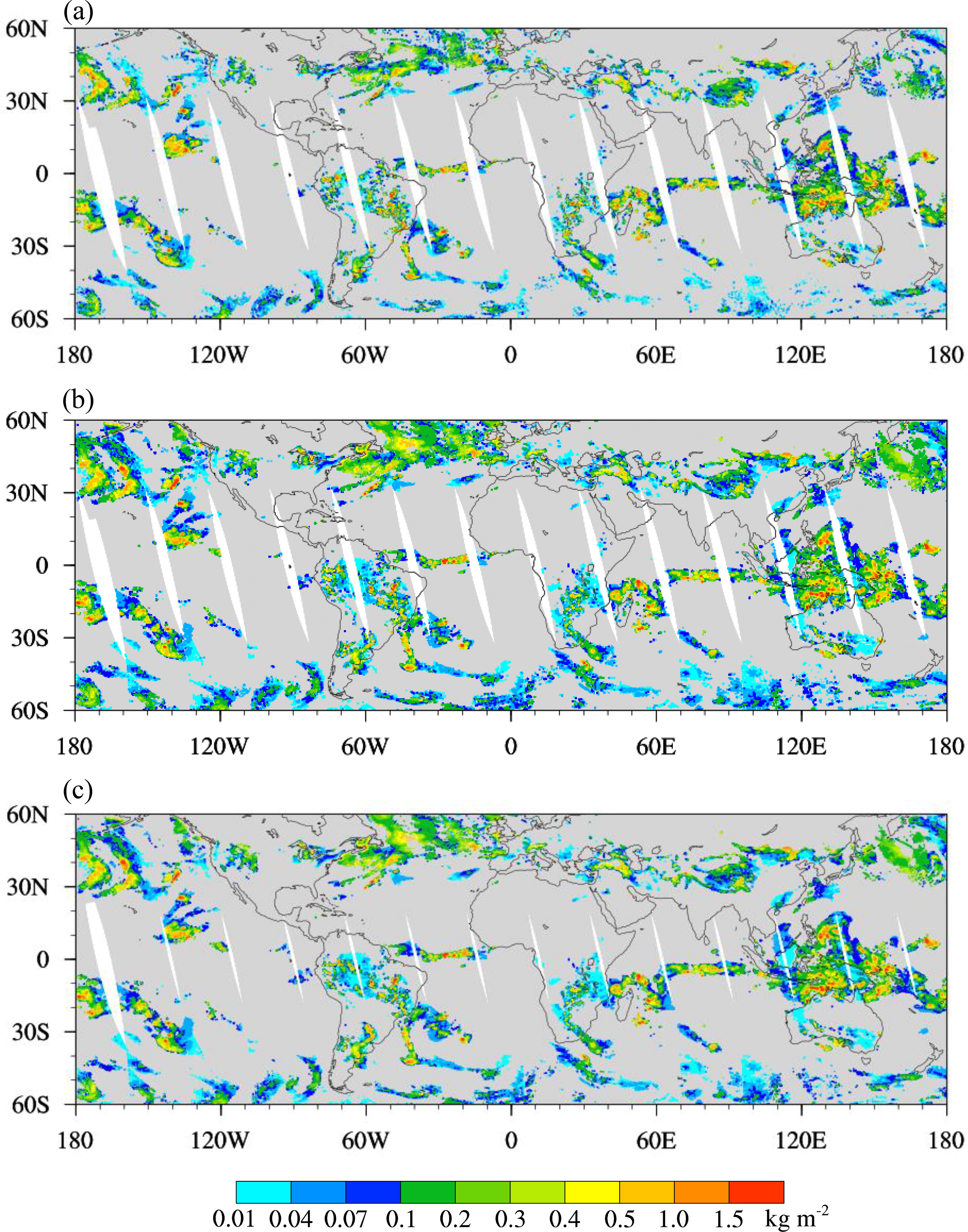
Fig. 9.
Same as Fig. 8 except that results for 4 February 2017 are shown.
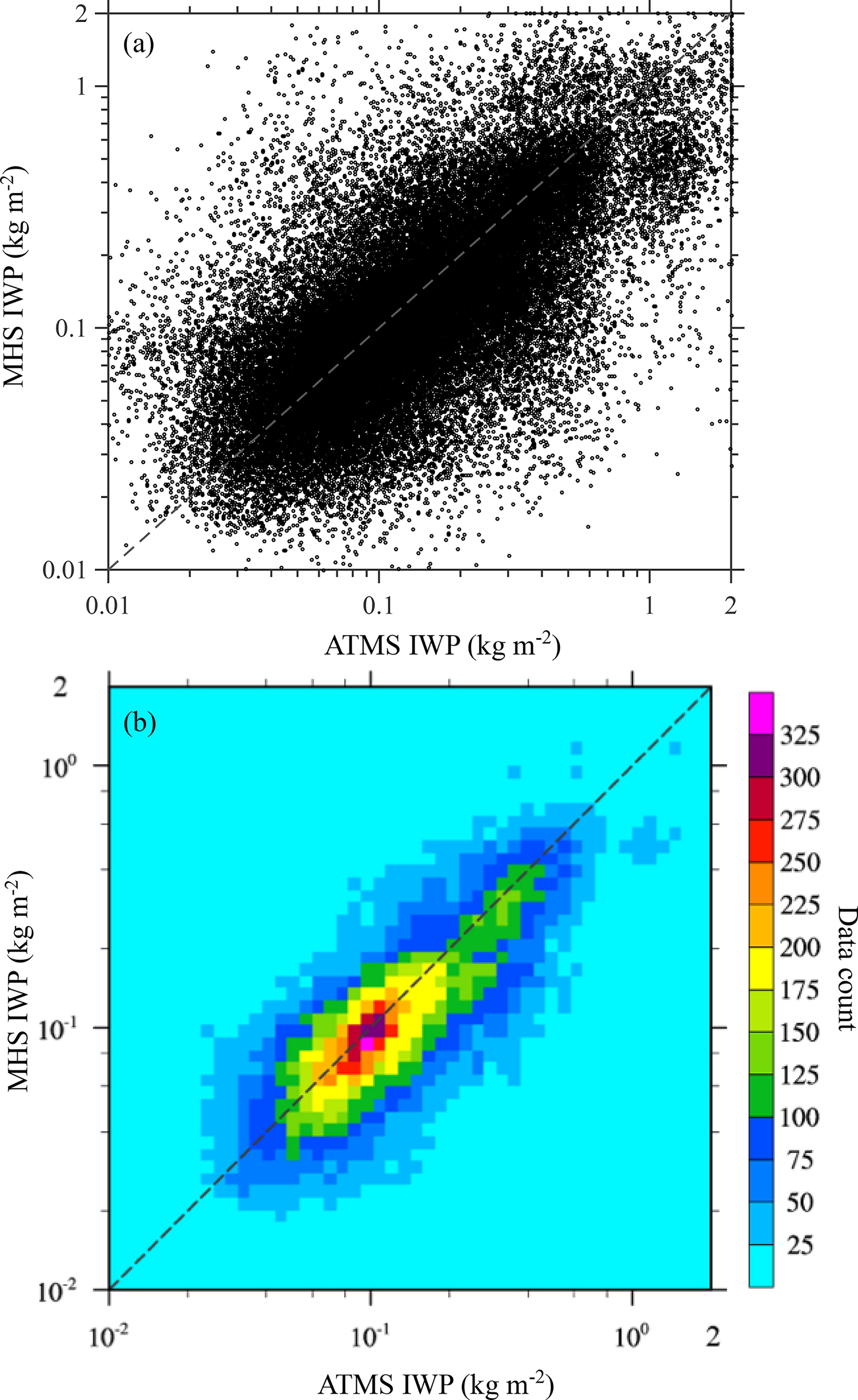
Fig. 10.
(a) MHS-derived IWP as a function of ATMS-derived IWP where the modified algorithm was applied to both retrievals and (b) associated data counts. Data are from between 60°S and 60°N on 12 December 2016 and 4 February 2017.
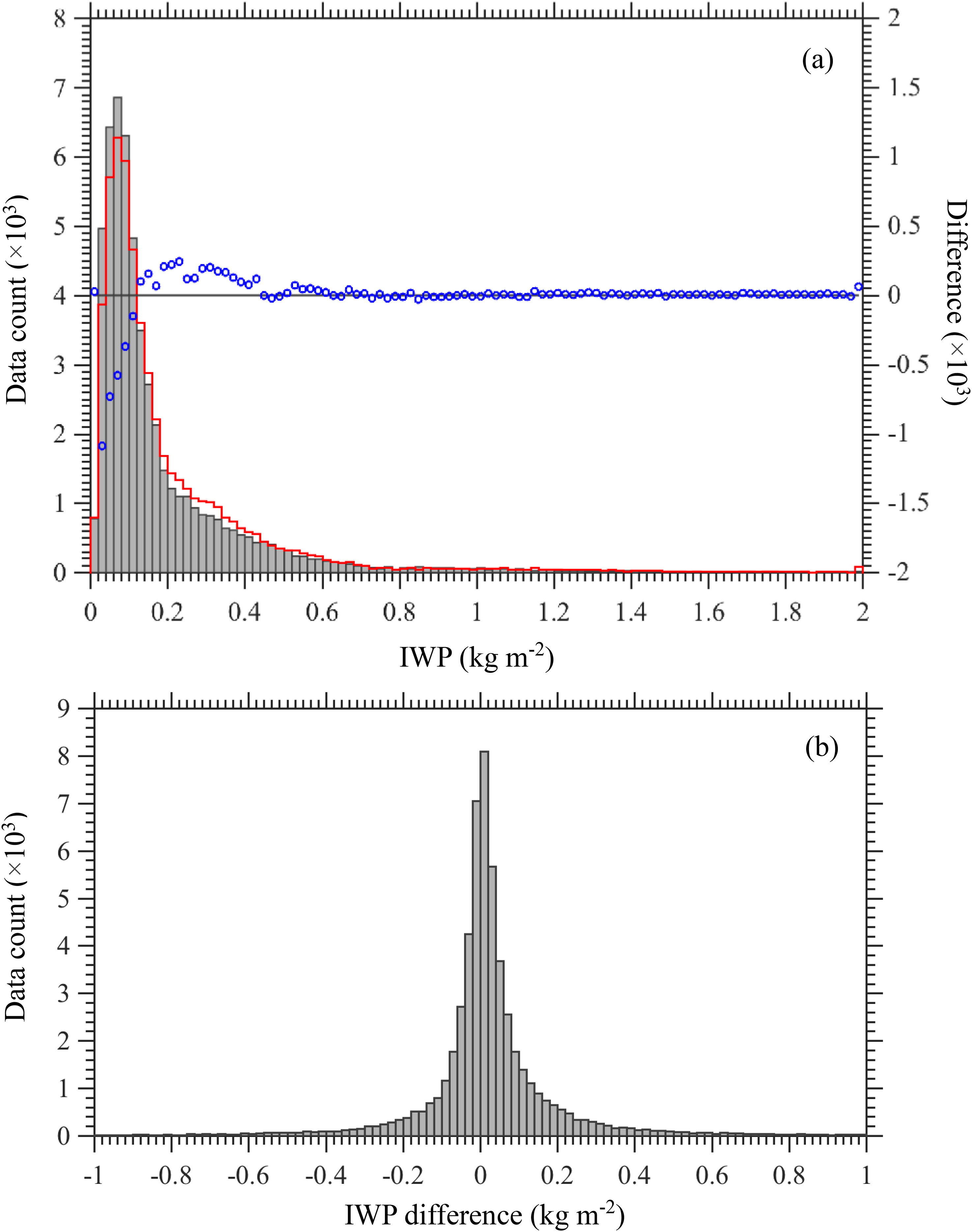
Fig. 11.
Data counts at 0.02 kg m−2 intervals of (a) collocated ATMS- (red) and MHS-derived (grey) IWPs calculated by the modified algorithm and the difference between the two data counts (right ordinate, blue circles), and of (b) differences between ATMS- and MHS-derived IWP. Data are on 12 December 2016 and 4 February 2017 between 60°S and 60°N.
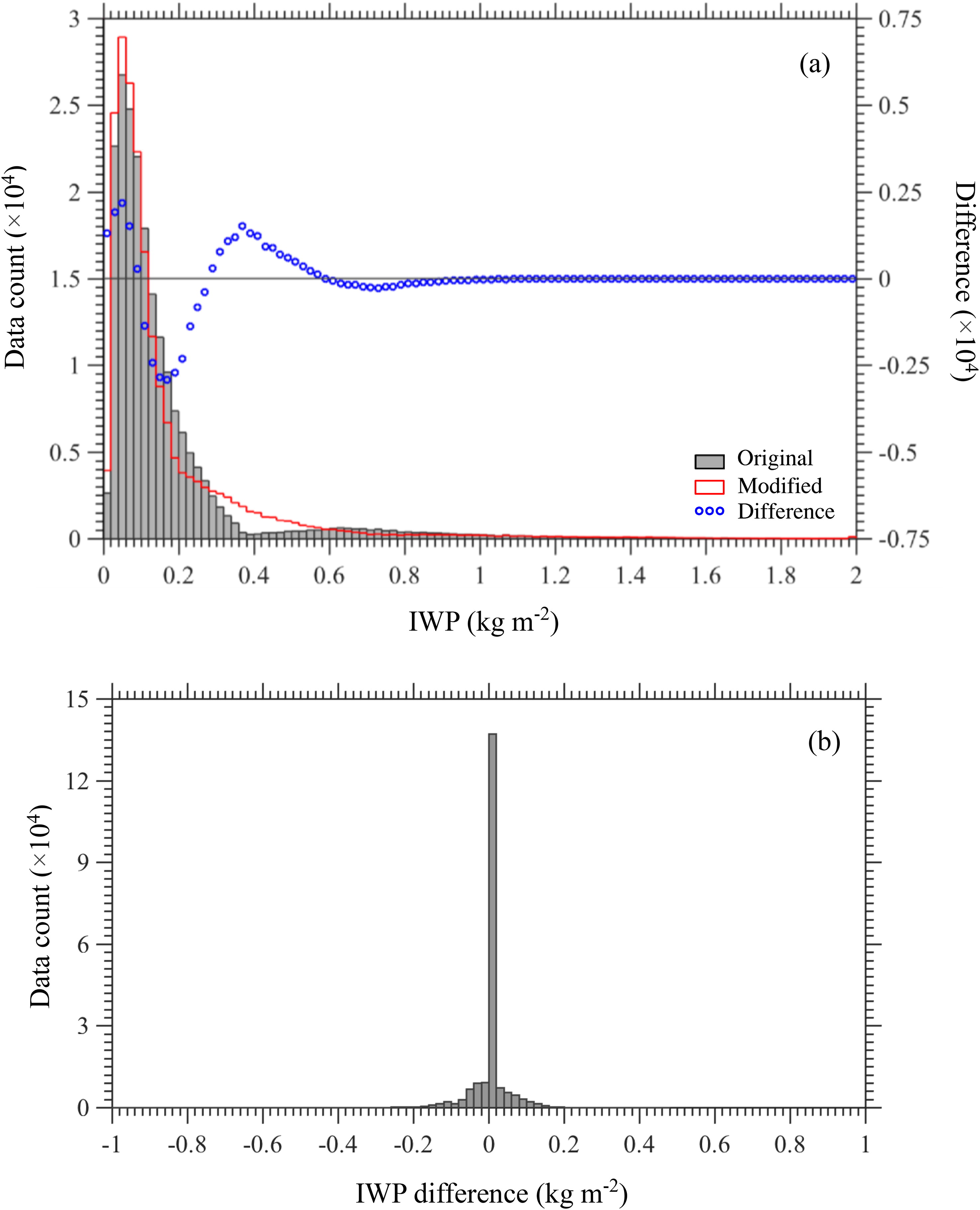
Fig. 12.
Data counts of (a) MHS-retrieved IWP at 0.02 kg m−2 intervals calculated using the modified (red) and the original (grey) algorithms and (b) differences between MHS-derived IWP with the modified and original algorithms for all data on 12 December 2016 and 4 February 2017.