Have a personal or library account? Click to login
‘The Equator–Pole grid system’: an overset grid system for the sphere, with an optimal uniformity property Cover

‘The Equator–Pole grid system’: an overset grid system for the sphere, with an optimal uniformity property

By:   
Open Access
|Jan 2018

Figures & Tables

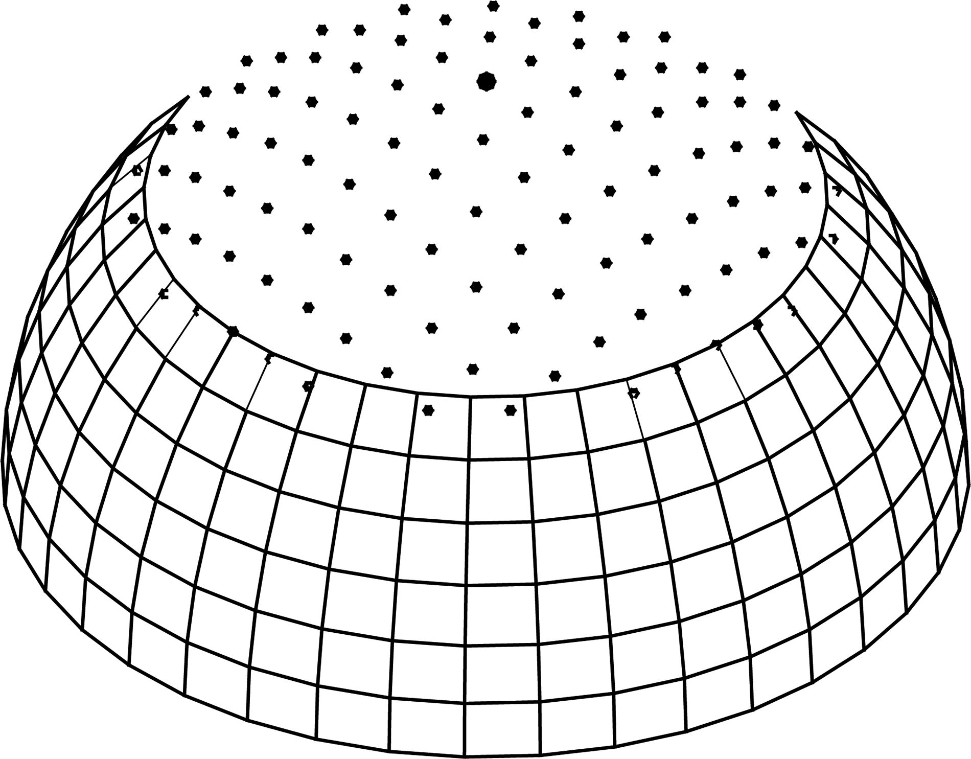
Fig. 1.

The grid system for a hemisphere, with N= 40 points around the equator, and without overlapping.
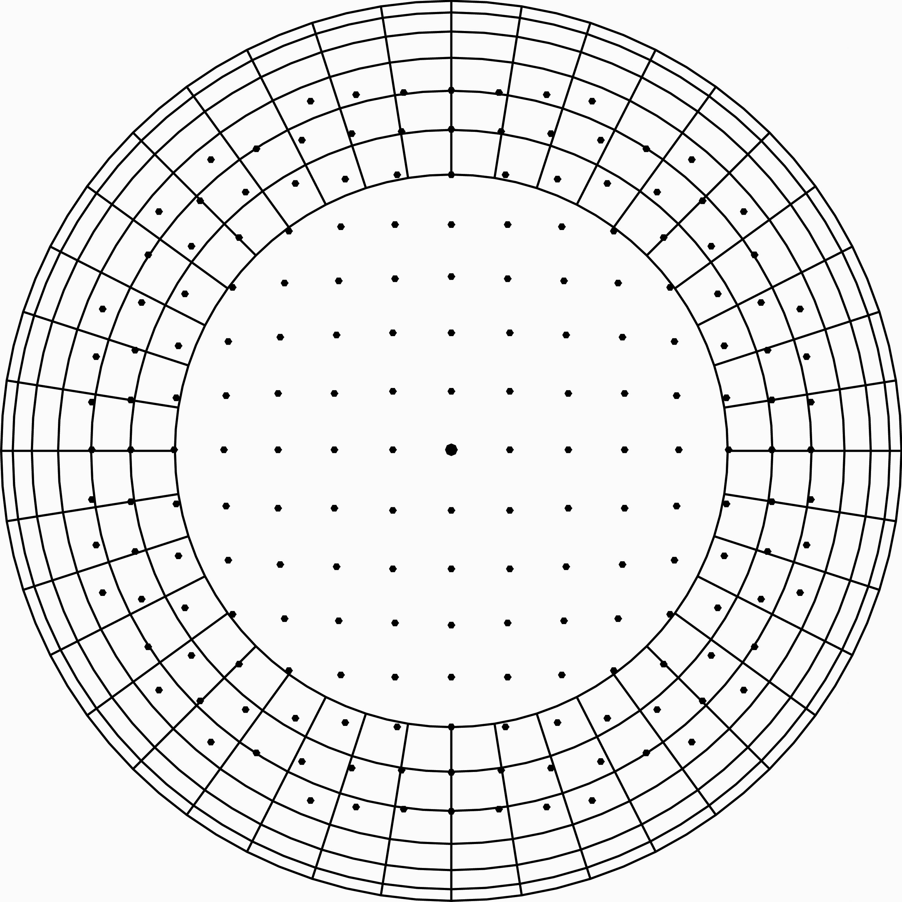
Fig. 2.

Orthogonally projected grid system on the equatorial plane, with overlapping corresponding to the centred 4th order method, and with N= 40.

Table 5.

The Rossby–Haurwitz wave: Relative changes of the total mass and energy.

relmass(1:7)1.27e − 72.43e − 72.59e − 72.94e − 71.55e − 7−1.01e − 7−3.31e − 7relmass(8:14)−3.59e − 7−2.92e − 7−1.35e − 72.13e − 89.88e − 81.32e − 8−1.81e − 7relenergy(1:7)4.24e − 41.70e − 33.32e − 34.47e − 35.01e − 35.46e − 35.70e − 3relenergy(8:14)5.67e − 35.70e − 35.56e − 35.16e − 35.12e − 35.34e − 35.15e − 3

[i] N = 360, 2p = 4, s = 2, c = 1.7e − 5, Δt=120s, Time =14 days.

Table 3.

Normalized errors for steady state geostrophic flow.

α108·c2psstc, (Ψ)stc,  2(Ψ)108·cmstc,  (Ψ)mstc,  2(Ψ)02.5427.4896e − 82.7333e − 82.02.3393e − 81.4434e − 84594.5424.5811e − 67.1803e − 715.09.8324e − 71.3341e − 7903.5423.3136e − 71.4239e − 73.53.3416e − 71.5007e − 700633.2131e − 101.0983e − 1001.7475e − 118.0196e − 12450634.9529e − 82.4985e − 903.7105e − 101.0249e − 10900635.7385e − 102.2245e − 1004.1246e − 102.0270e − 10

[i] N = 240, Δt=300s, Time =5 days, stc: = stereographic coord. and mstc: = modified stereographic coord.

Table 2.

Normalized errors for solid rotation of the Cosine bell.
α108·c2psminHmaxH(H)2(H)9098.542−7.44559.9906e + 27.4455e − 36.5382e − 387101.542−7.41759.9904e + 27.4175e − 36.5323e − 34543.042−6.29119.9758e + 26.2919e − 37.2938e − 39098.543−7.44419.9907e + 27.4452e − 36.5374e − 387102.043−7.41519.9904e + 27.4169e − 36.5313e − 39014.563−2.74159.9958e + 22.7466e − 32.3972e − 38712.063−2.73989.9956e + 22.7844e − 32.5172e − 38712.084−1.67301.0000e + 31.6995e − 32.2057e − 3

[i] N = 360, Δt=600s, Time =12 days, min(H).

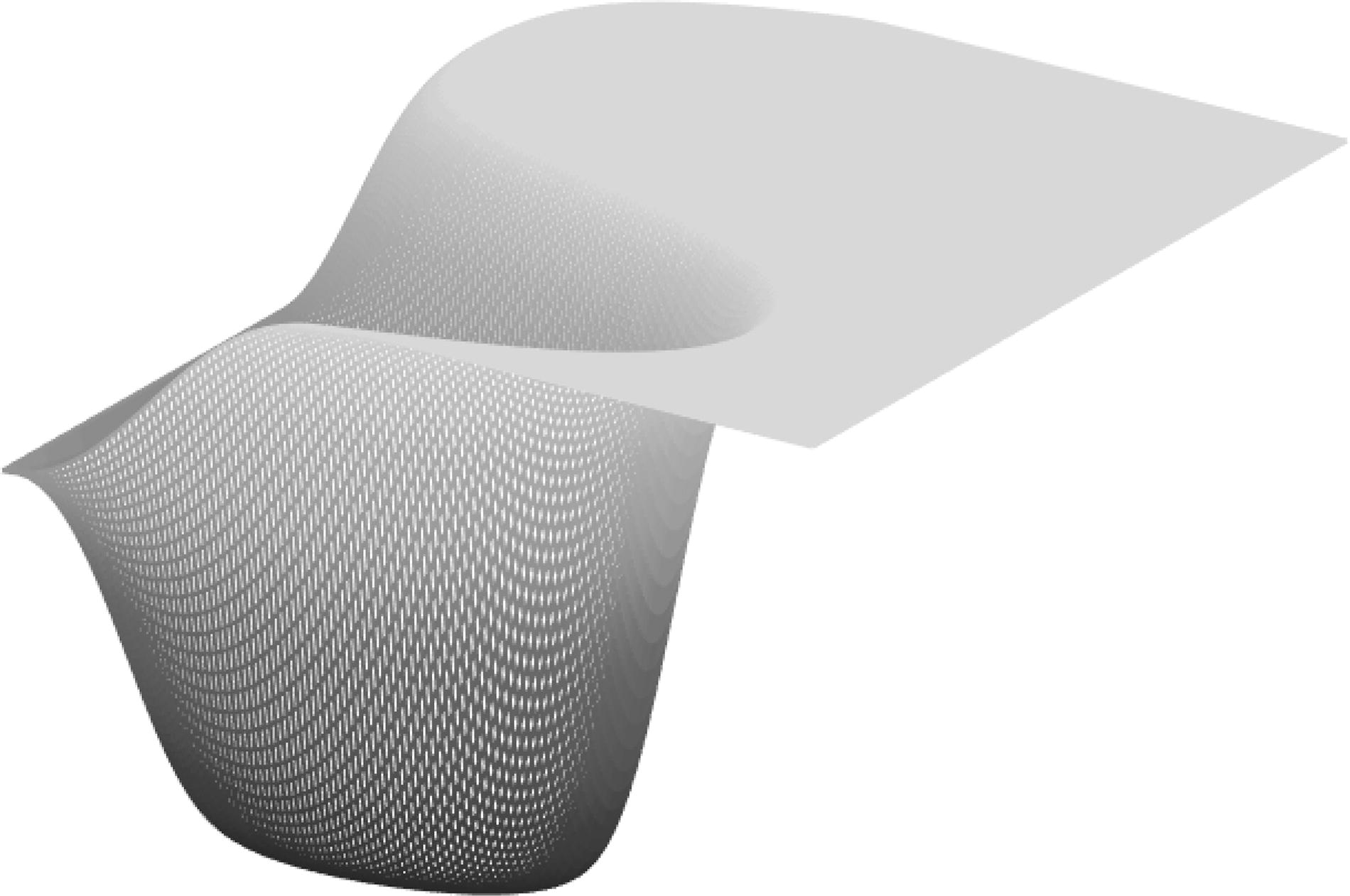
Fig. 3.

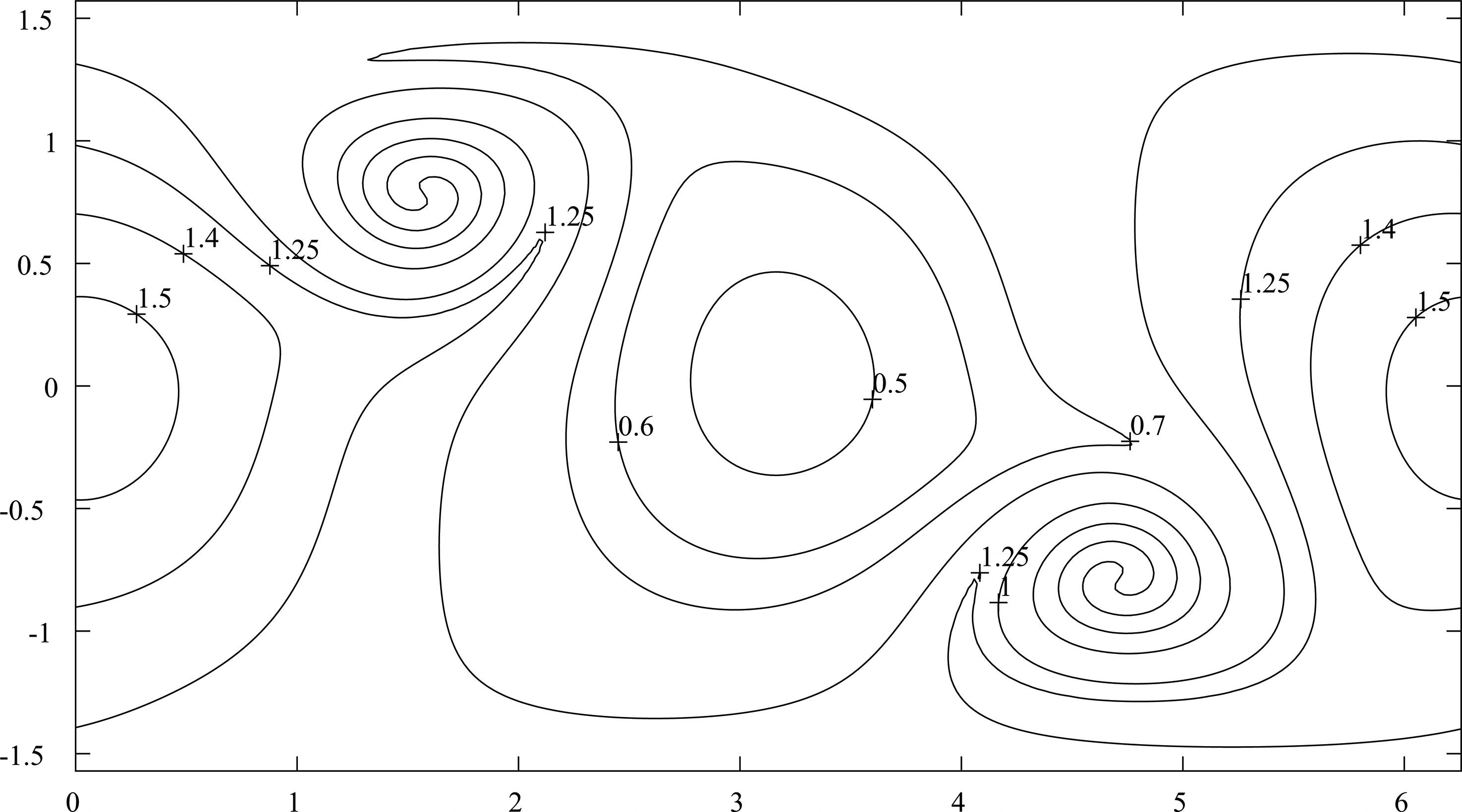
Contour curves for smooth deformational flow: α=45o, N = 240, 2p = 4 and Time=12 days.

Table 1.

Normalized errors for smooth deformational flow, stationary vortex.
α108·c2psminΨmaxΨ(Ψ)2(Ψ)01.0420.462951.53704.9954e − 36.4872e − 4453.5420.462991.53704.9587e − 35.6236e − 4901.6420.462971.53707.5553e − 31.0074e − 300.25630.462951.53701.1315e − 31.2714e − 4450.35630.462991.53701.1612e − 31.0952e − 4900.45630.462971.53702.1246e − 32.4623e − 4

[i] N = 240, Δt=400s, Time =12 days.

Fig. 4.

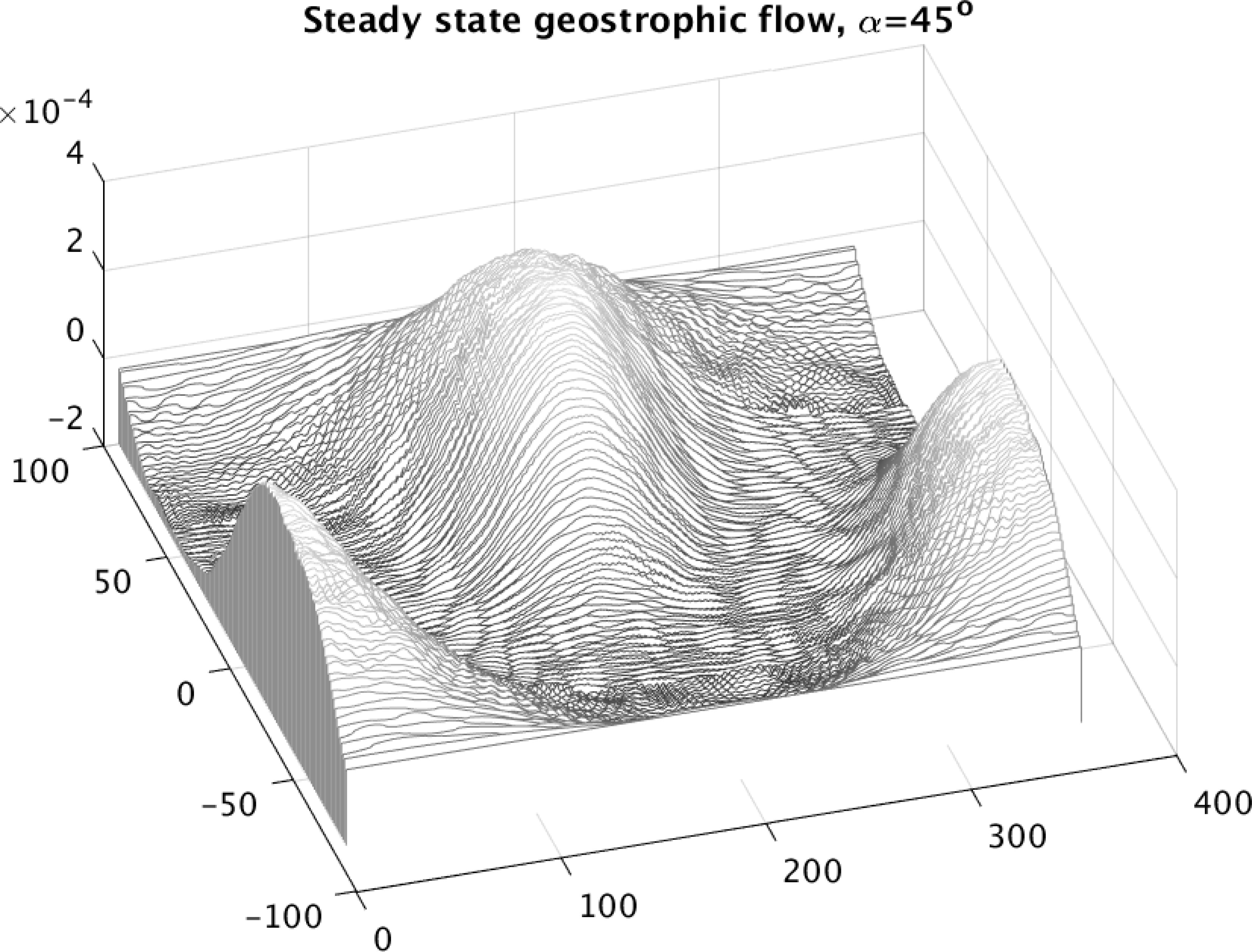
Absolute errors as function of lat–lon, with 2p = 6, N = 240 and Δt=300.

Fig. 5.

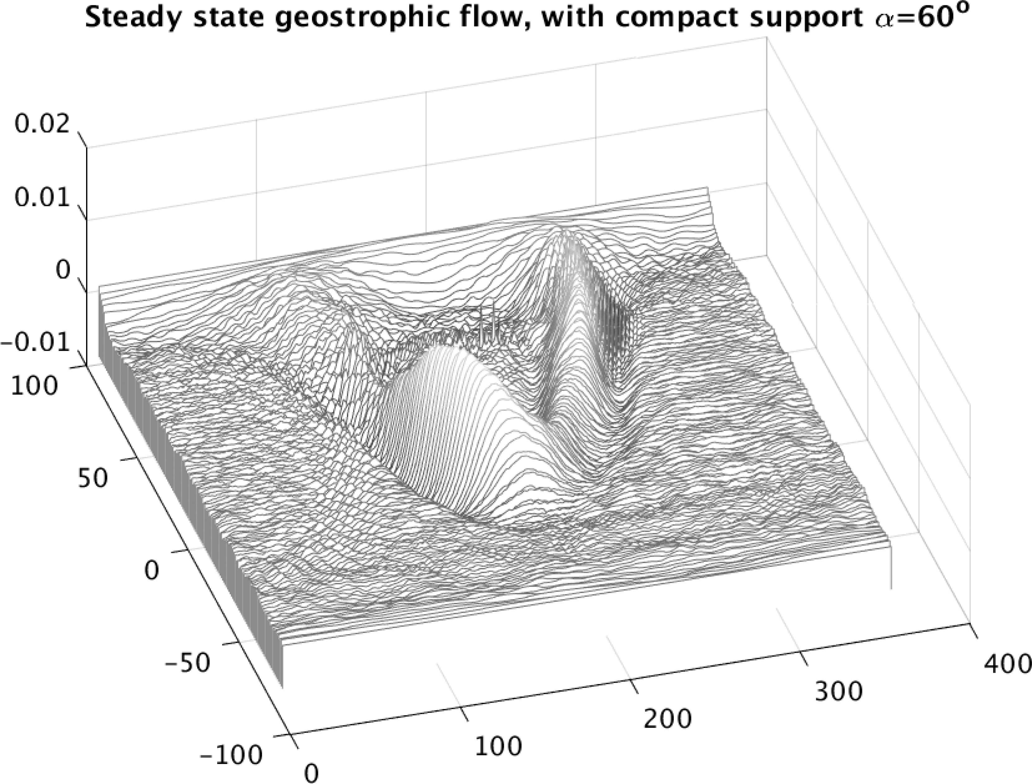
Geostrophic flow with compact support, with α=60° and N= 240.

Table 4.

Normalized errors for geostrophic flow with compact support.
α108·c2psminΨmaxΨ(Ψ)2(Ψ)07.0422.0572e + 42.9401e + 44.4288e − 61.1233e − 66010.5422.0572e + 42.9401e + 42.0841e − 54.0558e − 600632.0572e + 42.9401e + 47.5006e − 81.3479e − 8600632.0572e + 42.9401e + 42.8129e − 75.3725e − 8

[i] N = 240, Δt=300s, Time =5 days.

Fig. 6.

Absolute errors as function of lat–lon, with 2p = 6, N = 240 and Δt=300.

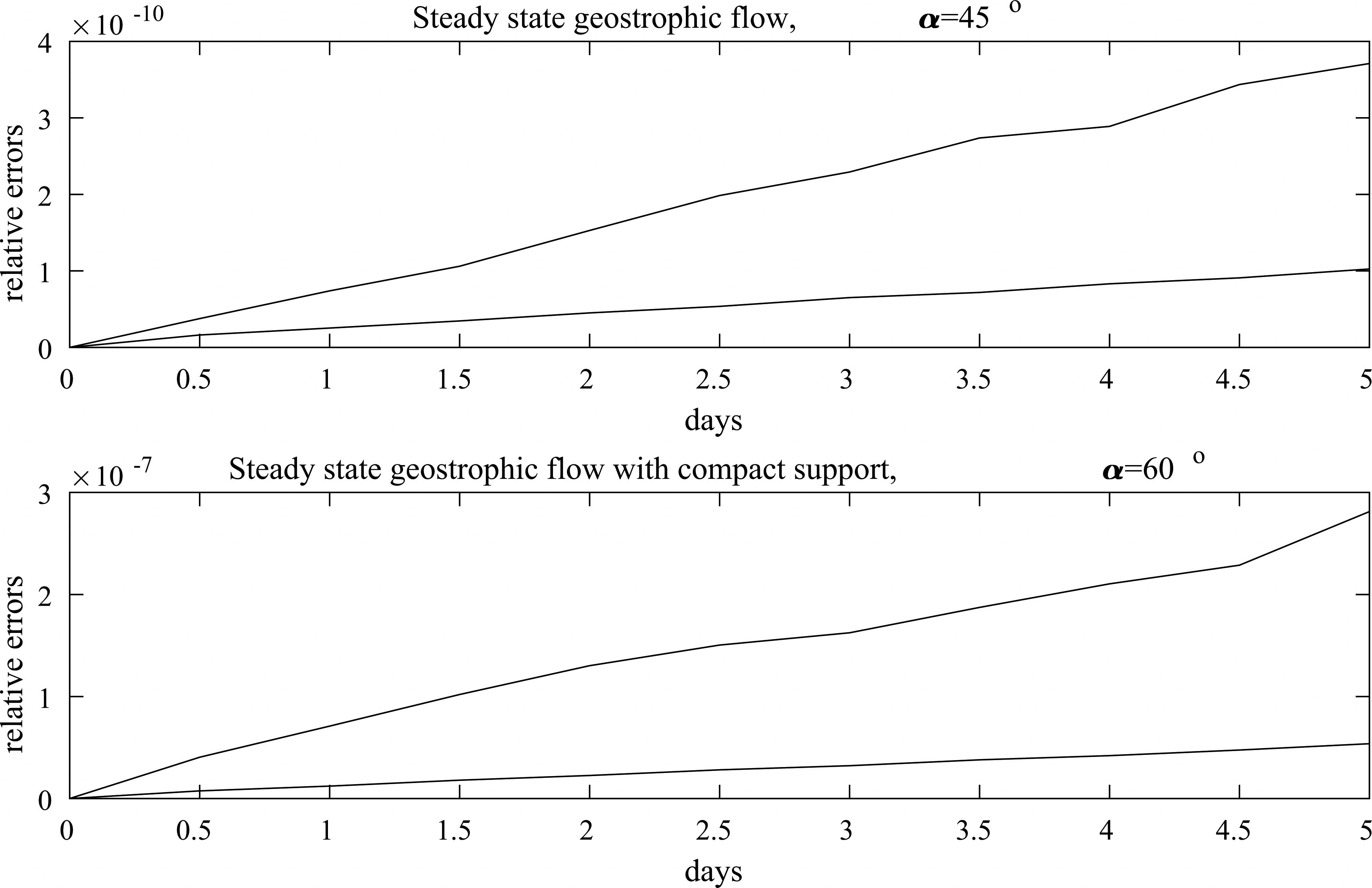
Fig. 7.

Test problems no. 2 and 3 from Williamson et al. (1992). In each panel the lower curve correspond to 2(Ψ) and the upper to (Ψ). In all cases 2p = 6, N = 240 and Δt=300.

Language: English
Page range: 1541373 - 1541373
Submitted on: Jan 12, 2018
Accepted on: Sep 28, 2018
Published on: Jan 1, 2018
Published by: Stockholm University Press
In partnership with: Paradigm Publishing Services

© 2018 Göran Starius, published by Stockholm University Press
This work is licensed under the Creative Commons Attribution 4.0 License.