
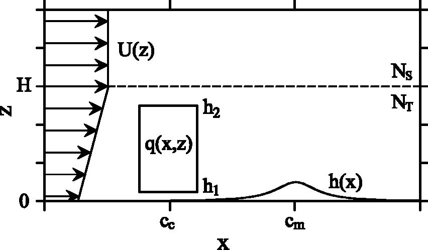
Fig. 1.
Structure of a two-layer atmosphere in the presence of convective forcing and a mountain considered in this study.
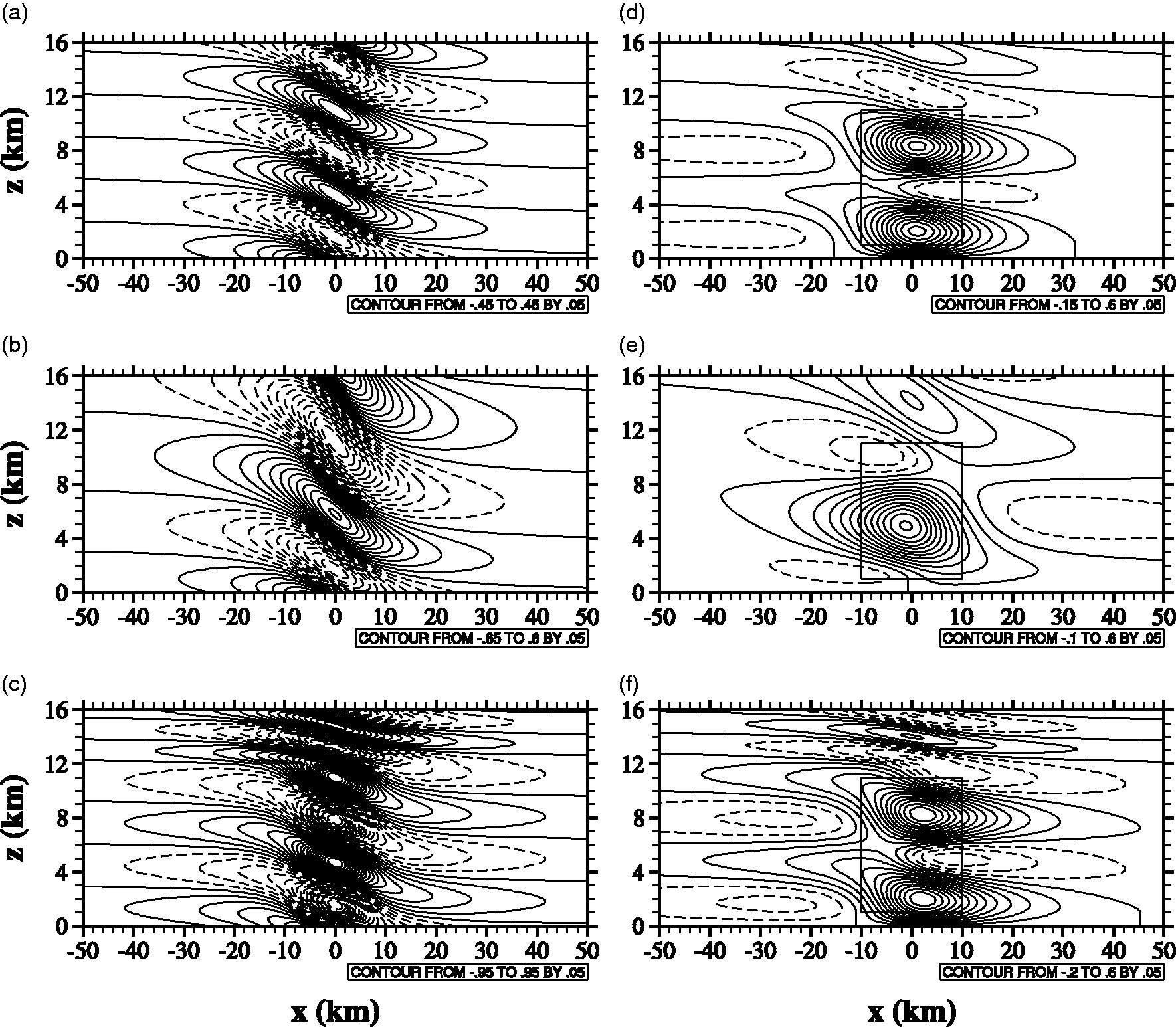
Fig. 2.
(a)–(c) Orographically and (d)–(f) convectively forced perturbation vertical velocity fields in the cases of N1U10 for (a) and (d), N1U20 for (b) and (e), and N2U10 for (c) and (f) with cm = 0 km and cc = 0 km. The rectangle in (d)–(f) represents the concentrated convective forcing region. The contour line information (unit: m s−1) is given at the bottom of each panel.
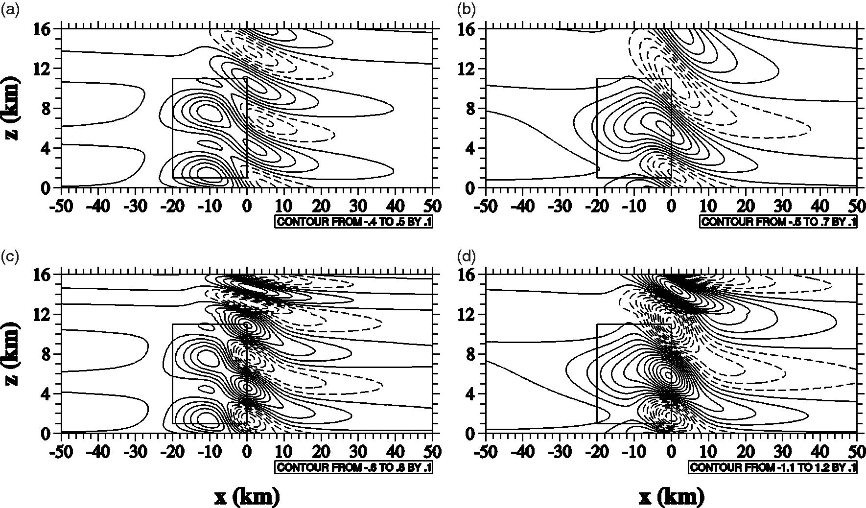
Fig. 3.
Perturbation vertical velocity fields in the cases of (a) N1U10, (b) N1U20, (c) N2U10, and (d) N2U20 with cc = –10 km. The rectangle in the troposphere represents the concentrated convective forcing region. The contour line information (unit: m s−1) is given at the bottom of each panel.
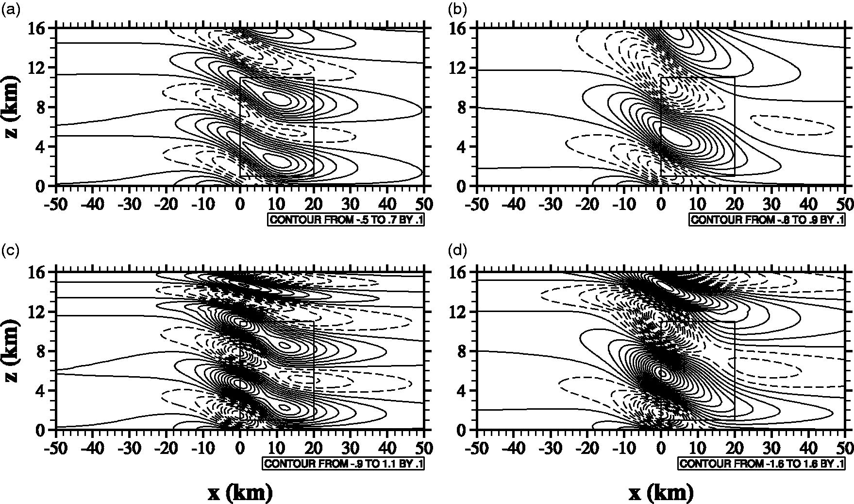
Fig. 4.
The same as Fig. 3 except for cc = 10 km.
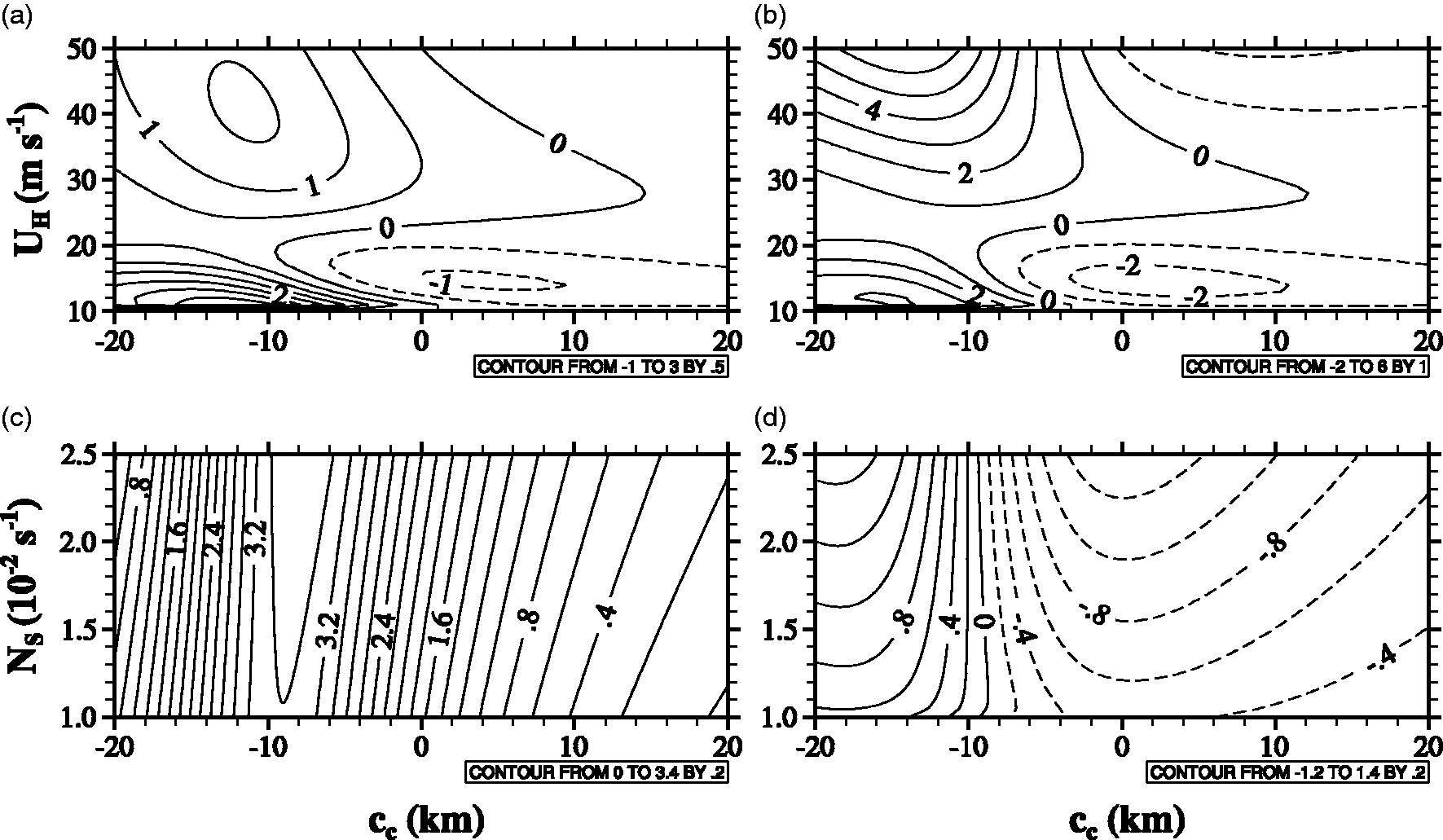
Fig. 5.
Fields of the ratio of the convectively forced perturbation vertical velocity to the orographically forced perturbation vertical velocity at (x, z) = (cm – am, h1) as a function of cc and UH in the cases of (a) N1Uyy and (b) N2Uyy and as a function of cc and NS in the cases of (c) NxU10 and (d) NxU20.
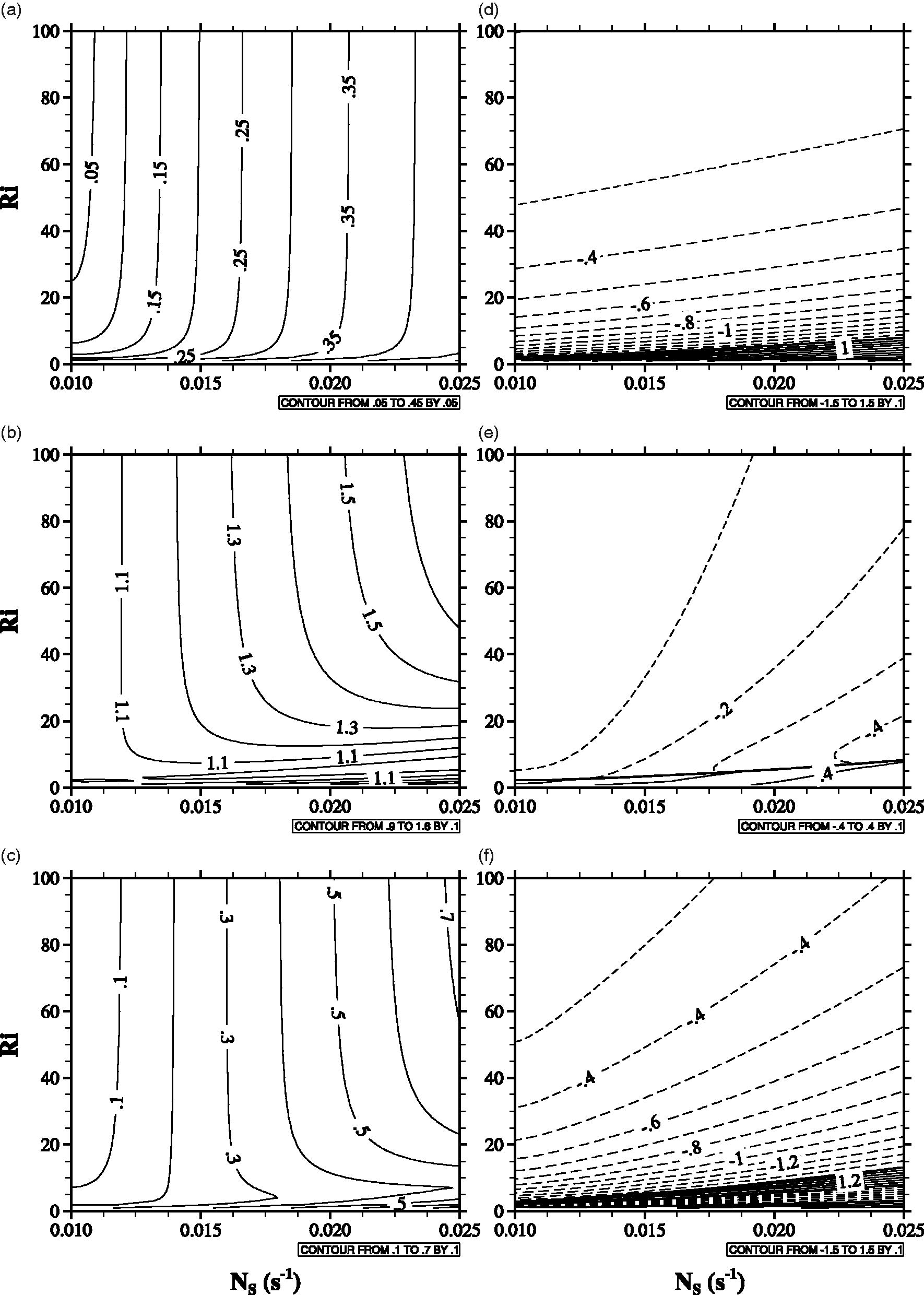
Fig. 6.
(a) R0, (b) R1, (c) R2, (d) θ0, (e) θ1, and (f) θ2 as a function of the stratospheric buoyancy frequency and the Richardson number. The values of θ0, θ1, and θ2 are in radian.
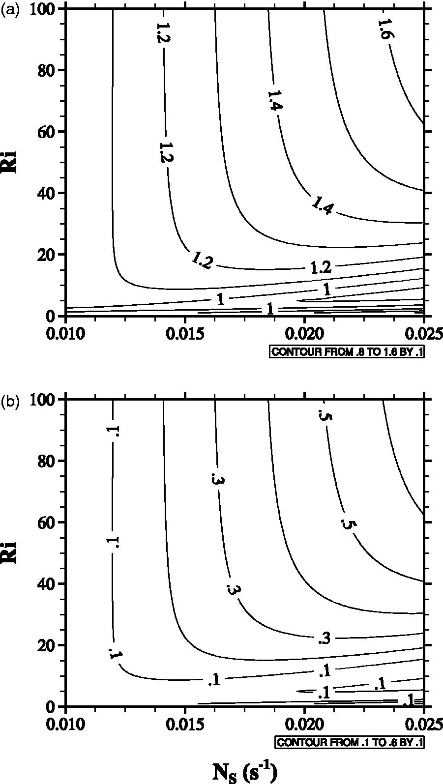
Fig. 7.
(a) R1cosθ1 and (b) R2cosθ2 as a function of the stratospheric buoyancy frequency and the Richardson number.
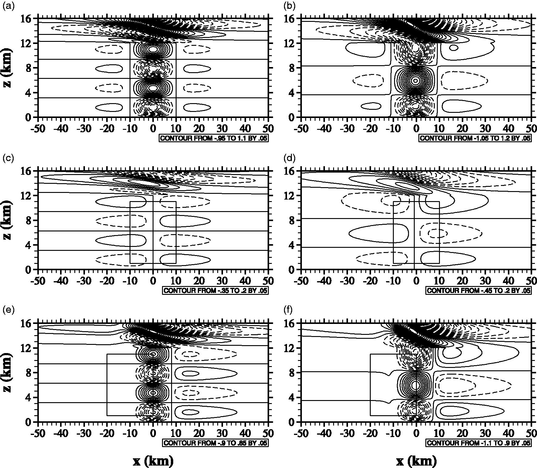
Fig. 8.
Differences in (a, b) orographically, (c, d) convectively, and (e, f) both orographically and convectively forced perturbation vertical velocity fields between the cases of N2U10 and N1U10 for the left column and between the cases of N2U20 and N1U20 for the right column. The centre of the convective forcing is located at x = 0 km in (c, d) and x = –10 km in (e, f). The contour line information (unit: m s−1) is given at the bottom of each panel.
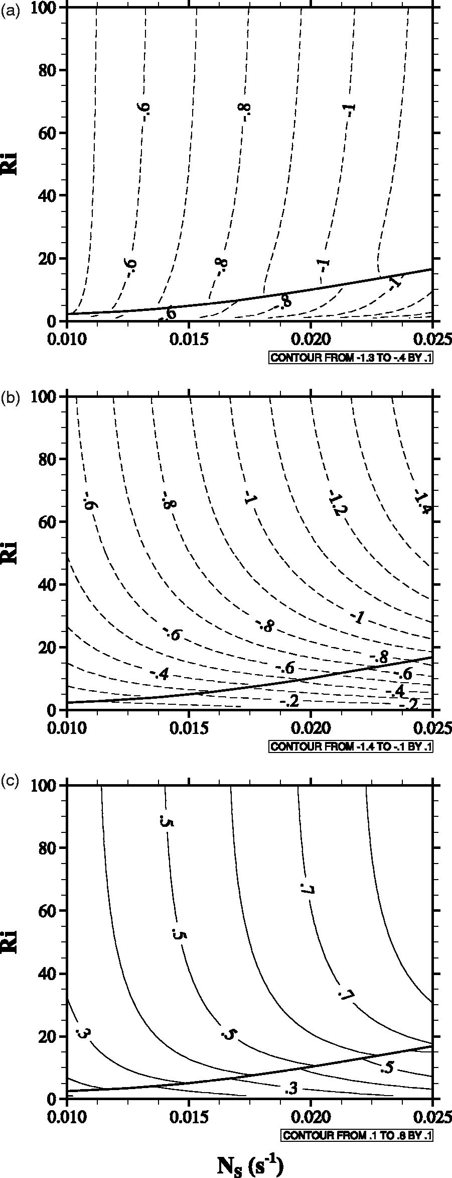
Fig. 9.
Momentum fluxes forced by the (a) mountain, (b) convection, and (c) orographic–convective interaction as a function of the stratospheric buoyancy frequency and the Richardson number. Here, cc – cm = –10 km is used.