
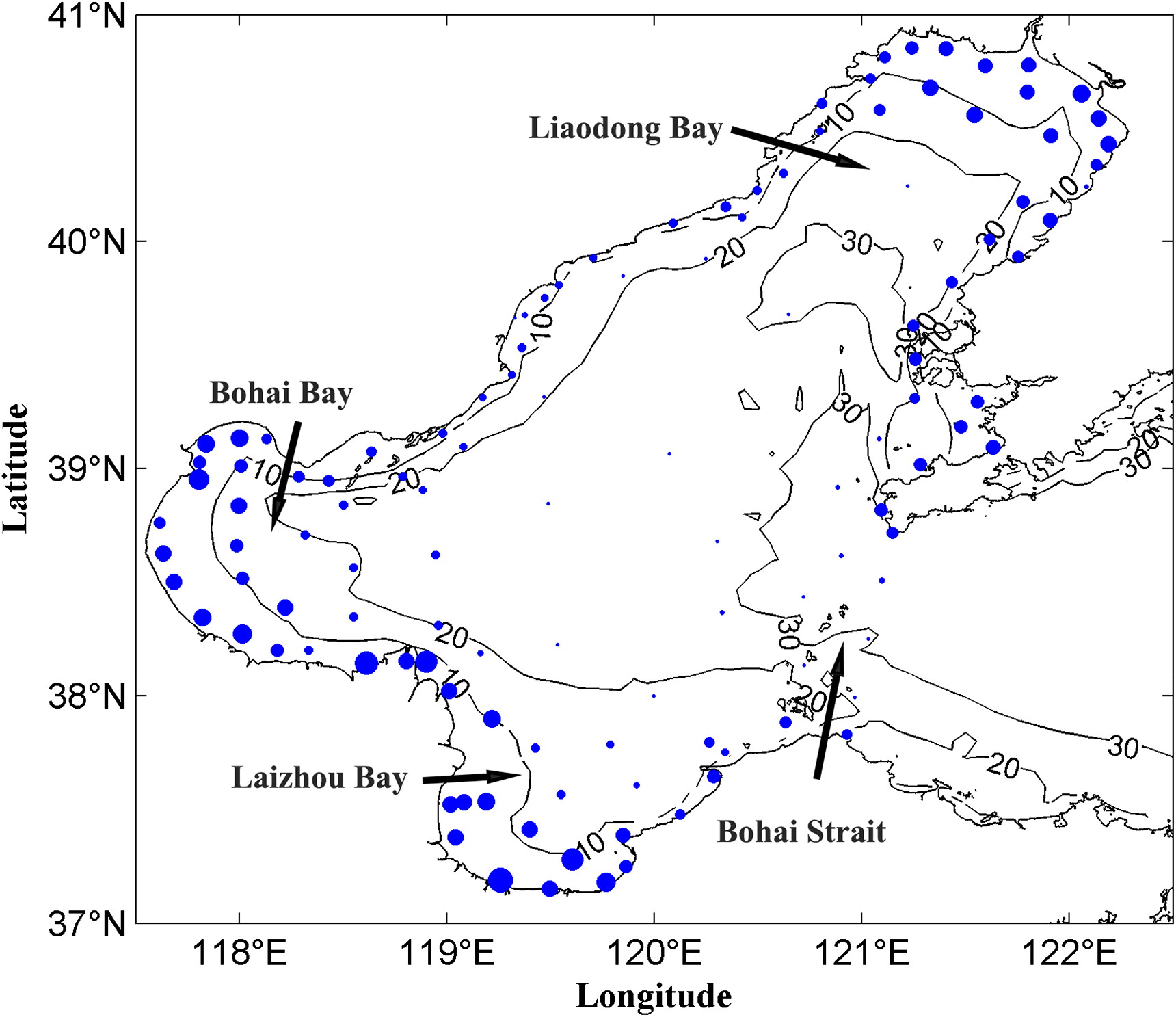
Fig. 1.
Topography of the Bohai Sea (depth in meters) and routine monitoring stations (blue dots) in May, 2009. Dots represent the location of stations and the size of each dot indicates the relative concentration of total nitrogen (TN) in May, 2009.
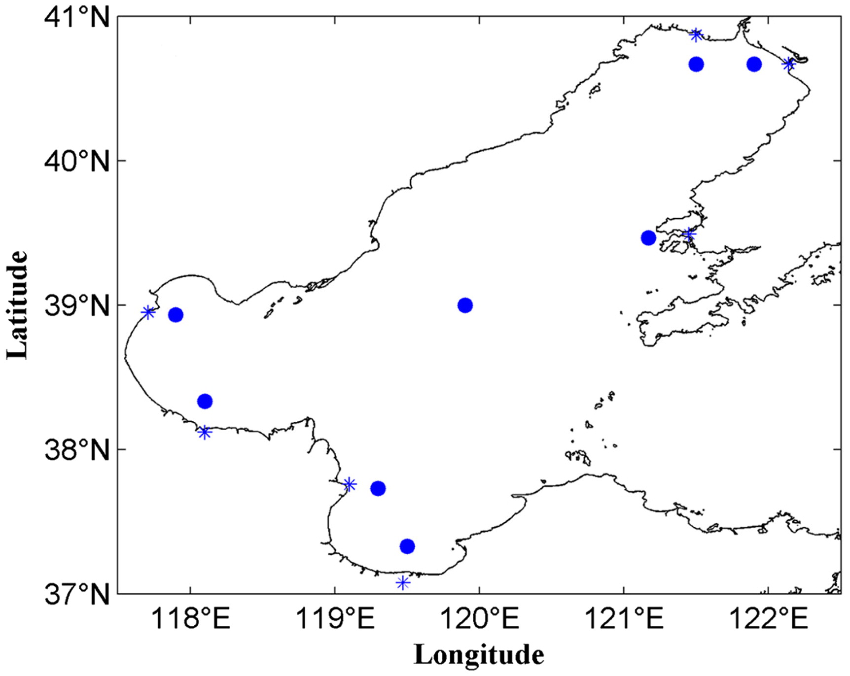
Fig. 2.
Locations of independent points. Dots represent independent points and stars represent estuaries.
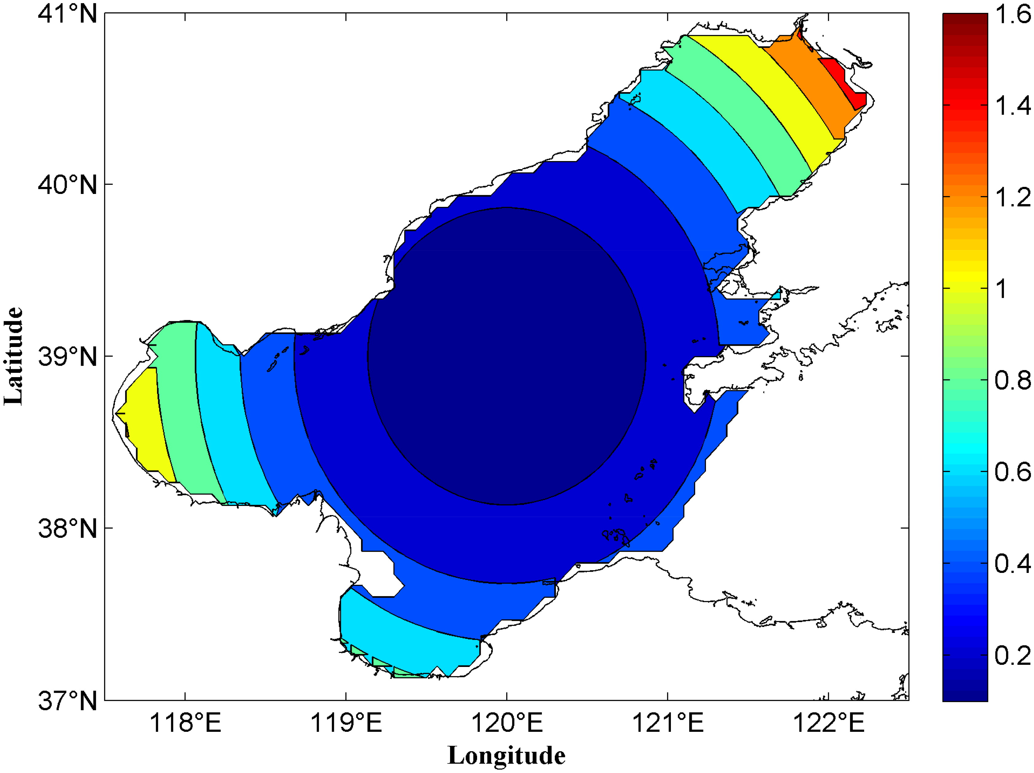
Fig. 3.
Assumed distribution of TN concentration (mg/L) in the Bohai Sea in ideal experiments.
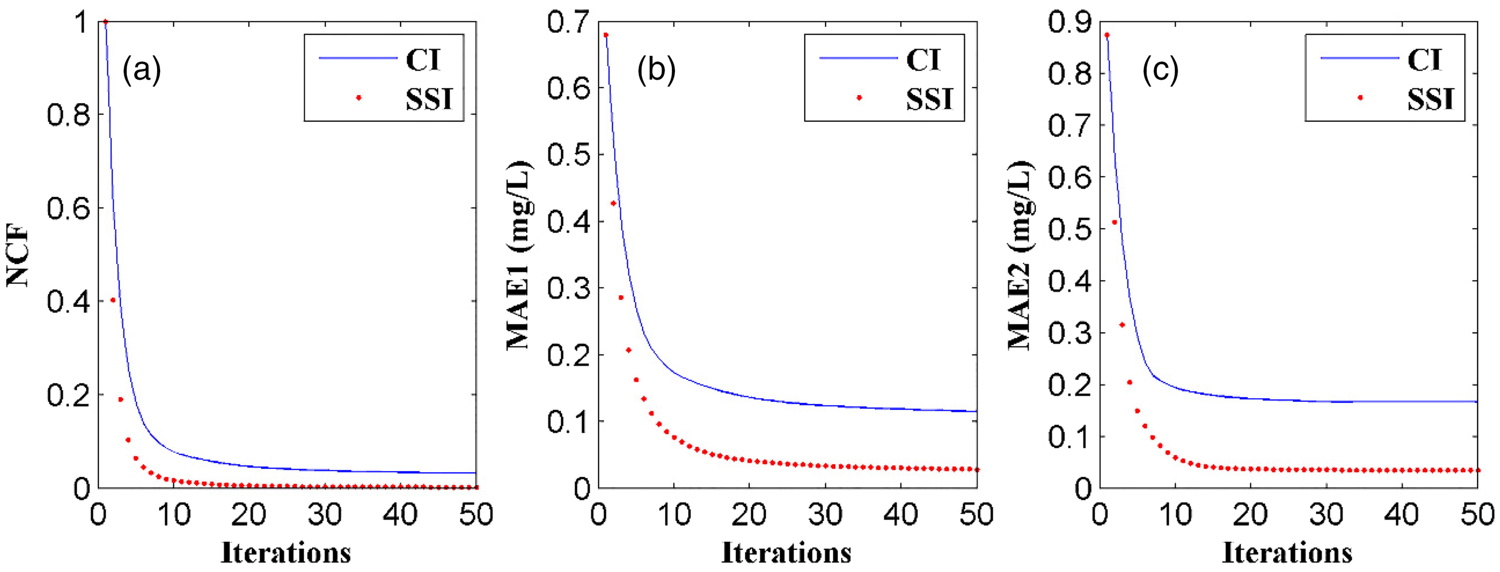
Fig. 4.
Results of ideal experiments. (a) The Normalized cost functions (NCFs), (b) mean absolute errors between simulated values and ‘observation’ at routine monitoring stations (MAE1) and (c) mean absolute errors between the inverted values and prescribed ones at all grid points in the computing area (MAE2s). Note that, in all panels, the blue solid lines are results by the Cressman interpolation (CI) and the red dashed lines are by the surface spline interpolation (SSI).
Table 1. Normalized cost functions (NCFs), mean absolute errors between simulated values and ‘observation’ at routine monitoring stations (MAE1s) and the mean absolute errors between the inverted values and prescribed ones at all grid points in the computing area (MAE2s) by the Cressman interpolation (CI) and the surface spline interpolation (SSI) in ideal experiments, respectively.
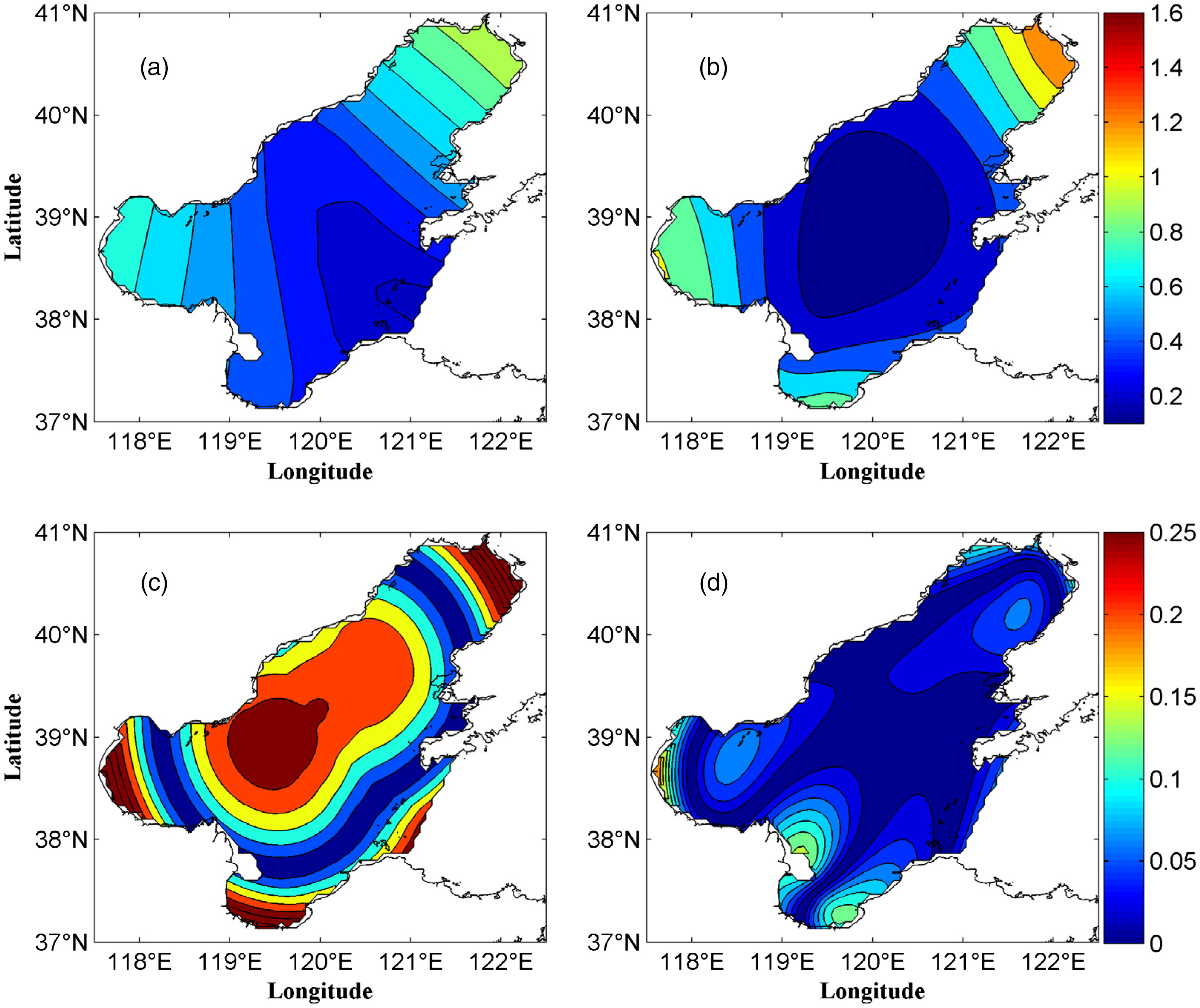
Fig. 5.
Results of ideal experiments. (a, b) The inverted initial distributions, (c, d) the absolute errors between the inverted initial distribution and the assumed shown in Fig. 3 (mg/L). Note that, (a, c) are results by the CI and (b, d) are those by the SSI.
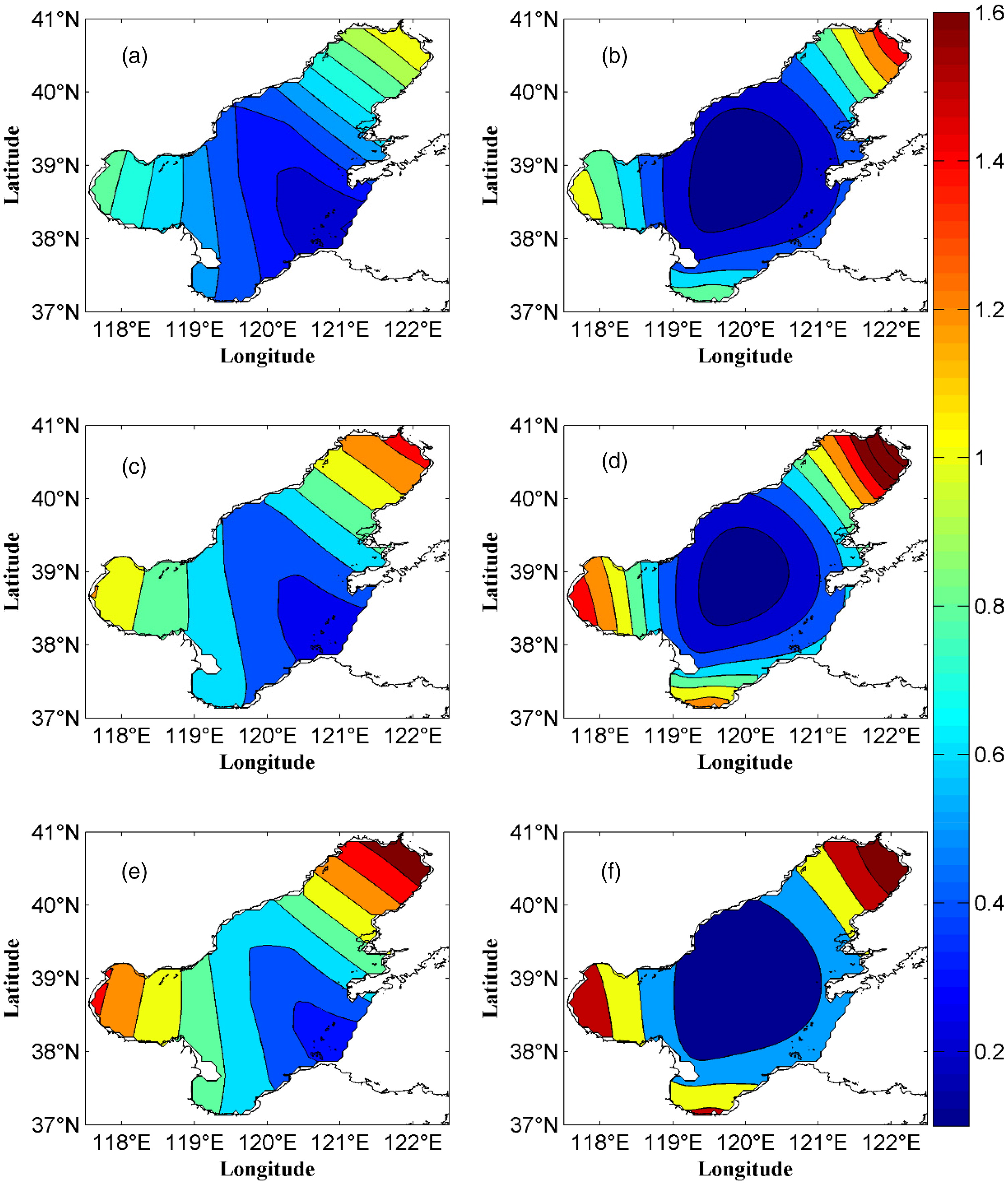
Fig. 6.
Inverted initial distributions of sensitivity experiments. (a, b) Inverted by assimilating ‘observations’ containing 10% errors, (c, d) containing 50% errors, (e, f) contains 80% errors. Note that, (a, c, e) are inverted by the CI and (b, d, f) are by the SSI.
Table 2. MAE2s by the CI and the SSI through assimilating ‘observations’ containing with percentage errors in sensitivity experiments, respectively.
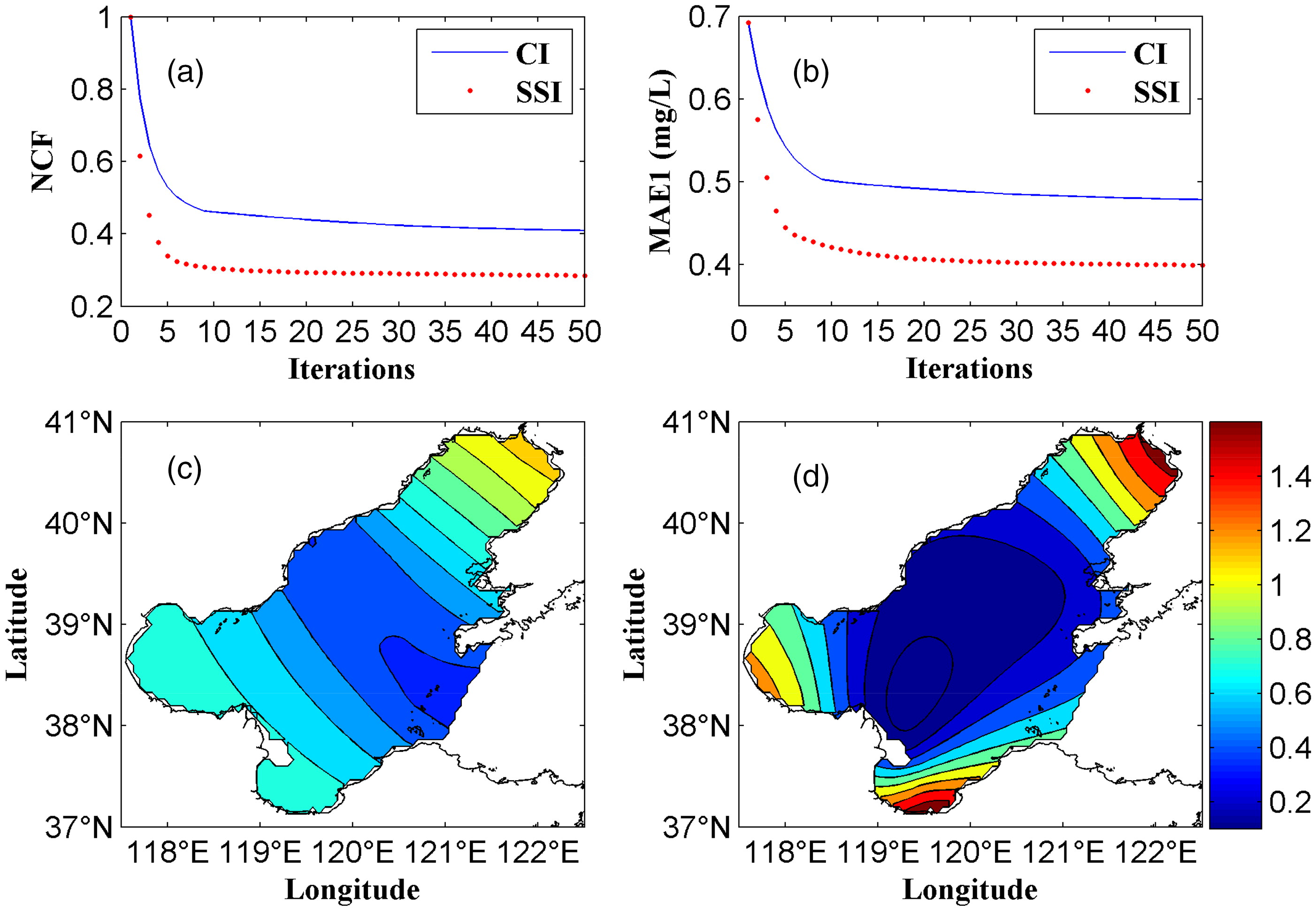
Fig. 7.
Results of practical experiments. (a) The NCFs, (b) the MAE1s, (c) the initial distribution inverted by the CI, (d) the initial distribution inverted by the SSI.
Table 3. MAE1s by the CI and the SSI in practical experiments, respectively.
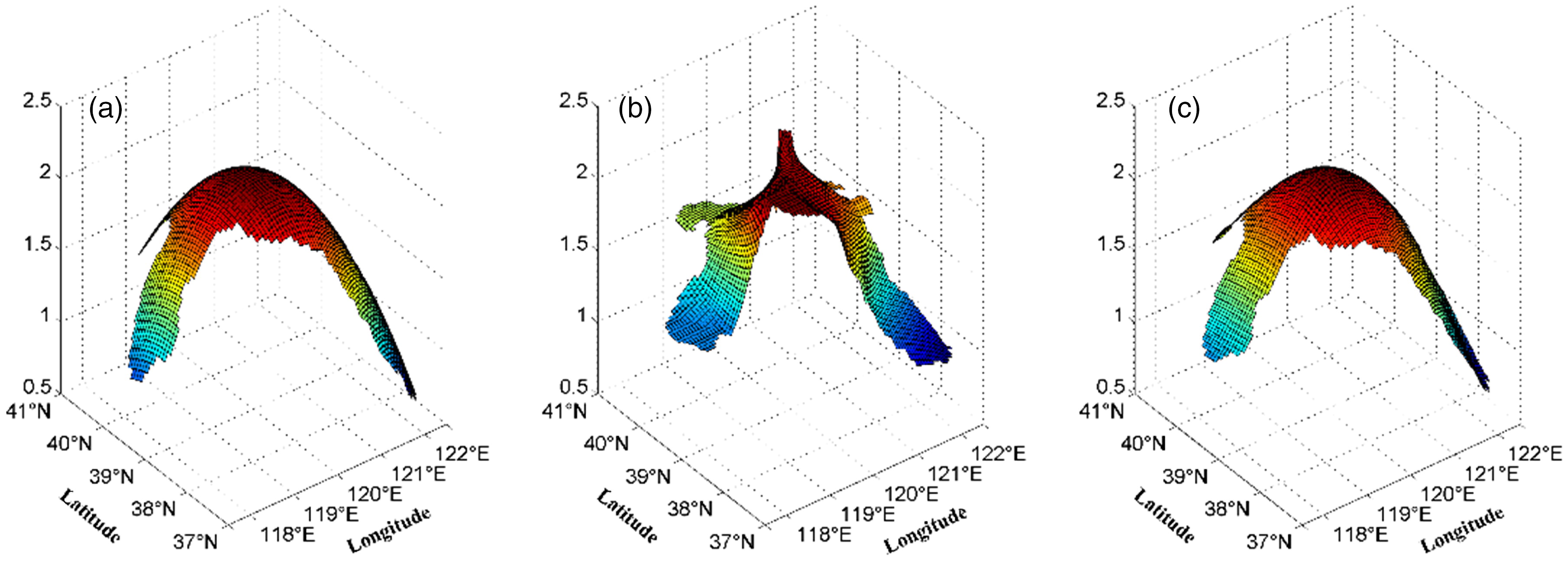
Fig. 8.
Comparison of the interpolation results by the CI and SSI. (a) The prescribed surface, (b) the interpolation result by the CI, (c) the interpolation result by the SSI.