
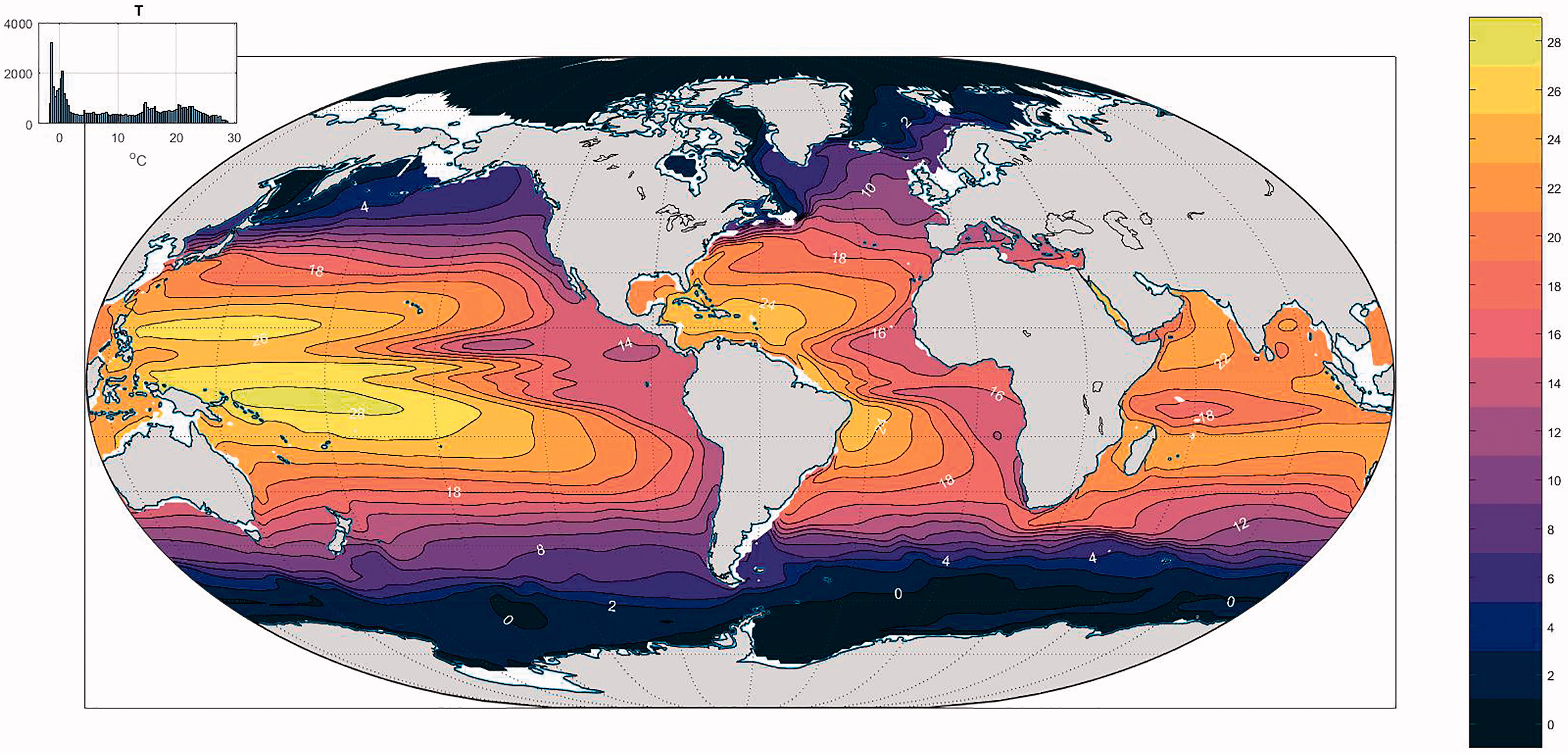
Fig. 1.
Twenty-year mean temperature at 105 m (°C). Inset shows the multi-modal histogram of values. The gyre structure is dominant and regarded here as a deterministic element of the field (Fukumori et al., 2018).
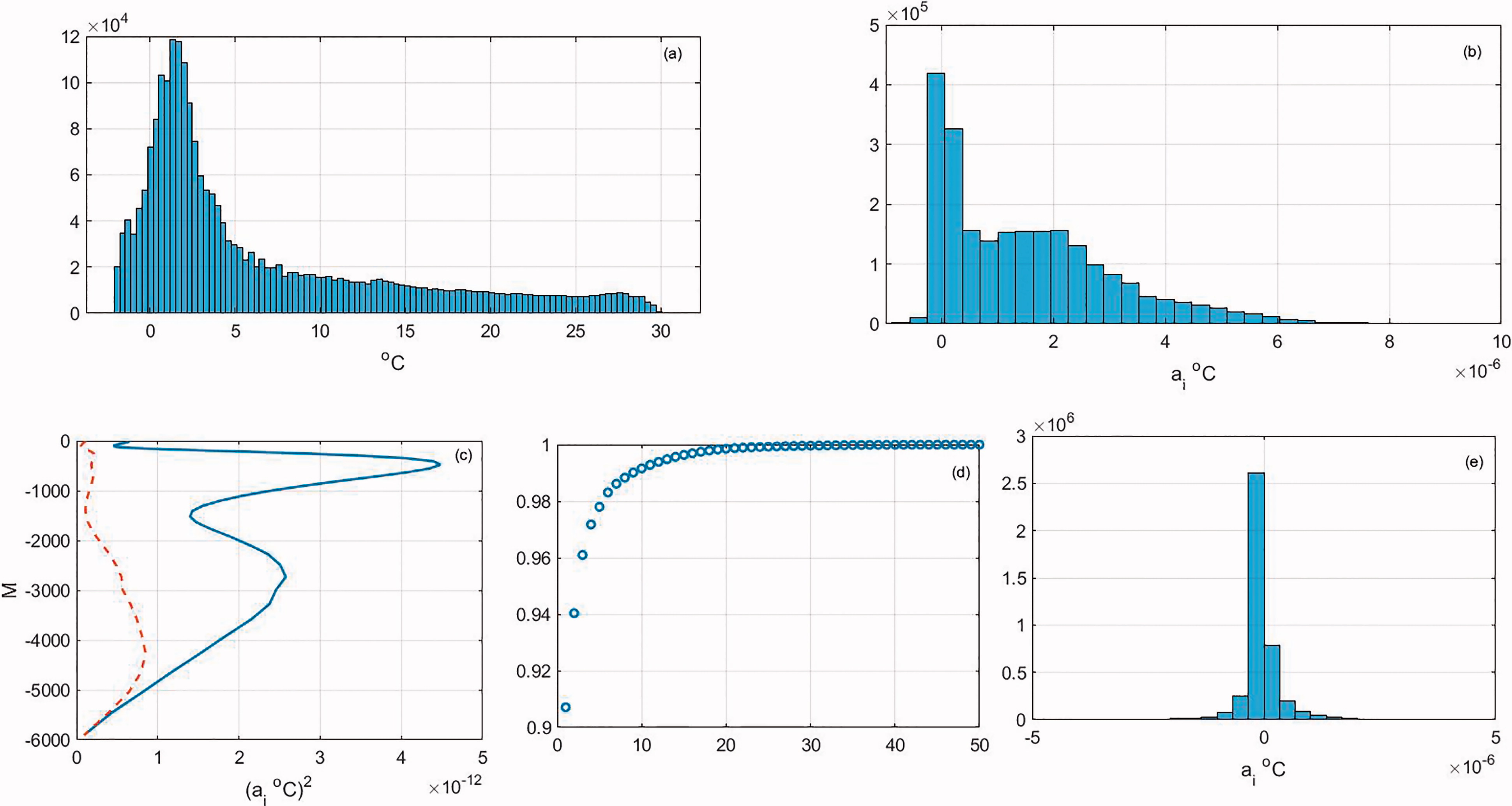
Fig. 2.
(a) Histogram of temperature values occuring at each grid point in the 20-year average temperature. (b) Same as (a) except each value is weighted by the fractional volume corresponding to the particular grid point. (c) Variance with depth of the weighted temperatures in (b) before (solid line) and after (dashed line) removal of the lowest singular vector pair. (d) Cumulative sum of squared singular vectors for time-mean temperature field. (e) Histogram of values in the residual after removal of the q = 1 singular value pair and which is unimodal without a dominating skewness.
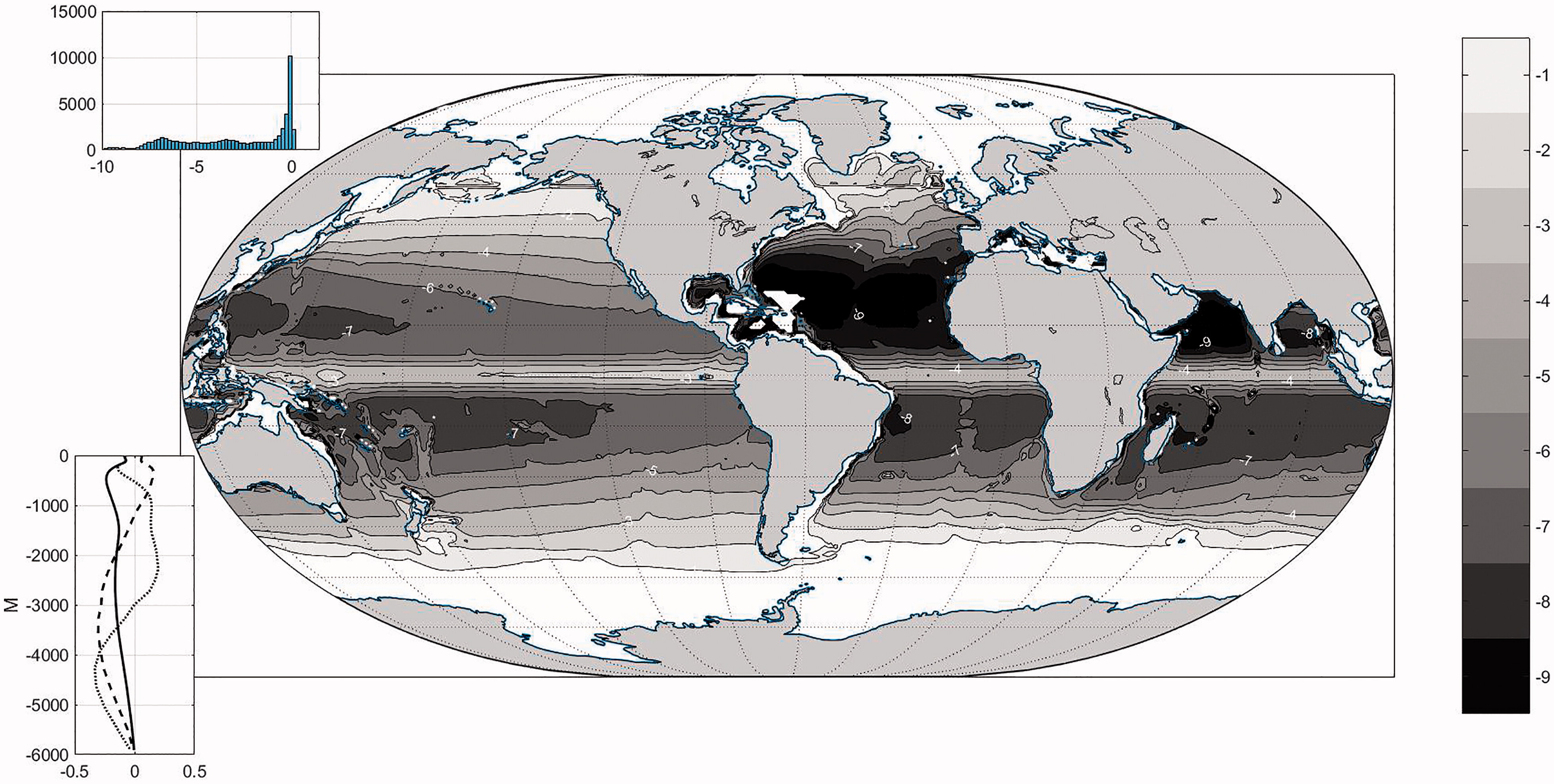
Fig. 3.
Chart of the values of singular vector for volume weighted time mean temperatures as a function of position (multiplied by 1000). All contours shown are negative. Lower left inset displays (solid curve) the corresponding value with depth of (solid curve) along with (dashed) and (dotted). Note that almost everywhere so that the product, is almost everywhere a positive volume weighted temperature. Upper left inset is the histogram of values and which is far from unimodal.
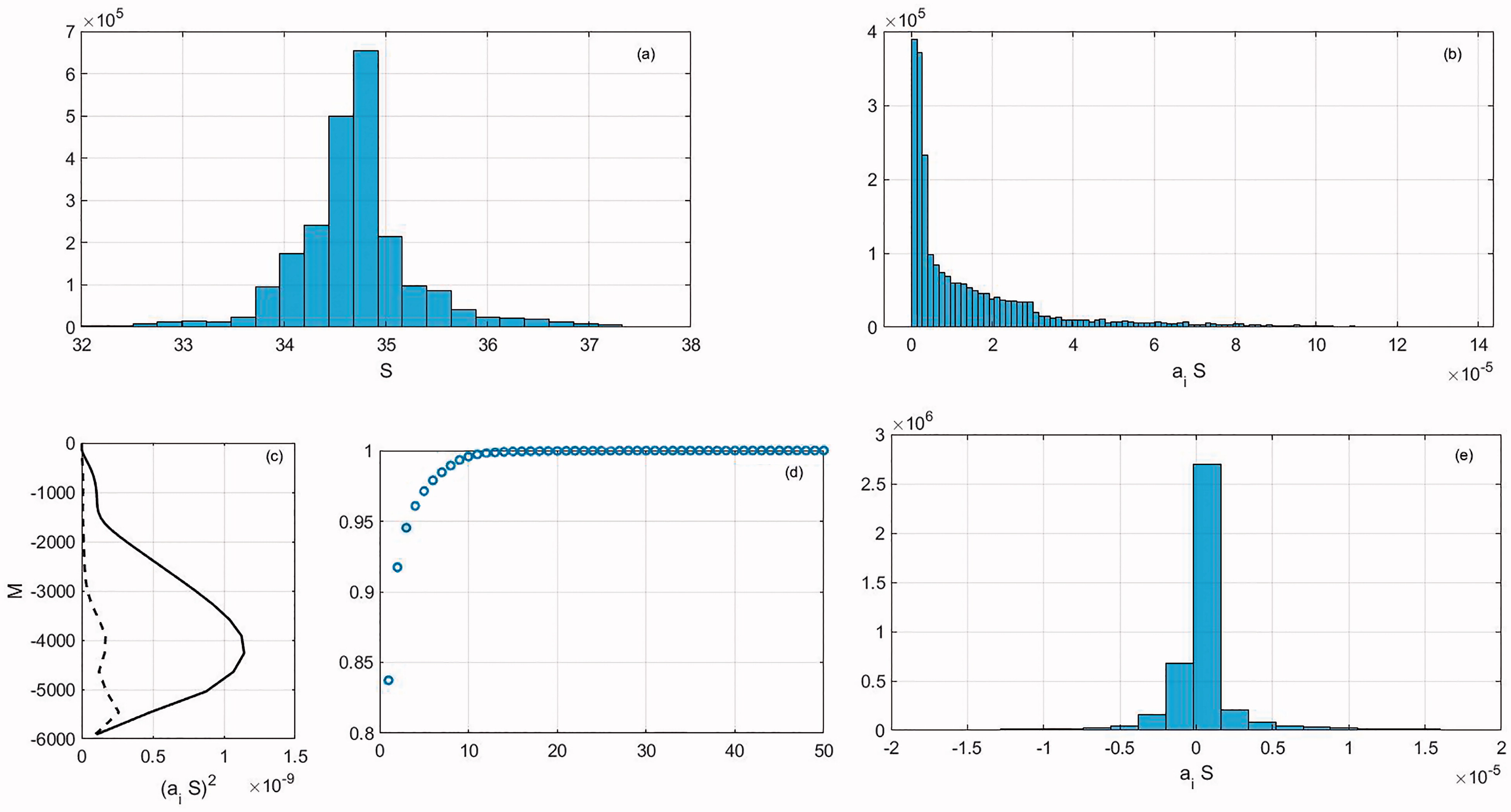
Fig. 4.
(a) Histogram of salinity values, (dimensionless) on each model grid point. (b) Same as (a) except each salinity value is weighted by its corresponding fractional volume represented (. (c) Variance of ( with depth (solid curve) and after removing q = 2 pairs of singular vectors. (d) Normalized accumulating sum of singular values of . (e) Histogram of volume weighted residuals after removing q = 2 singular vector pairs.
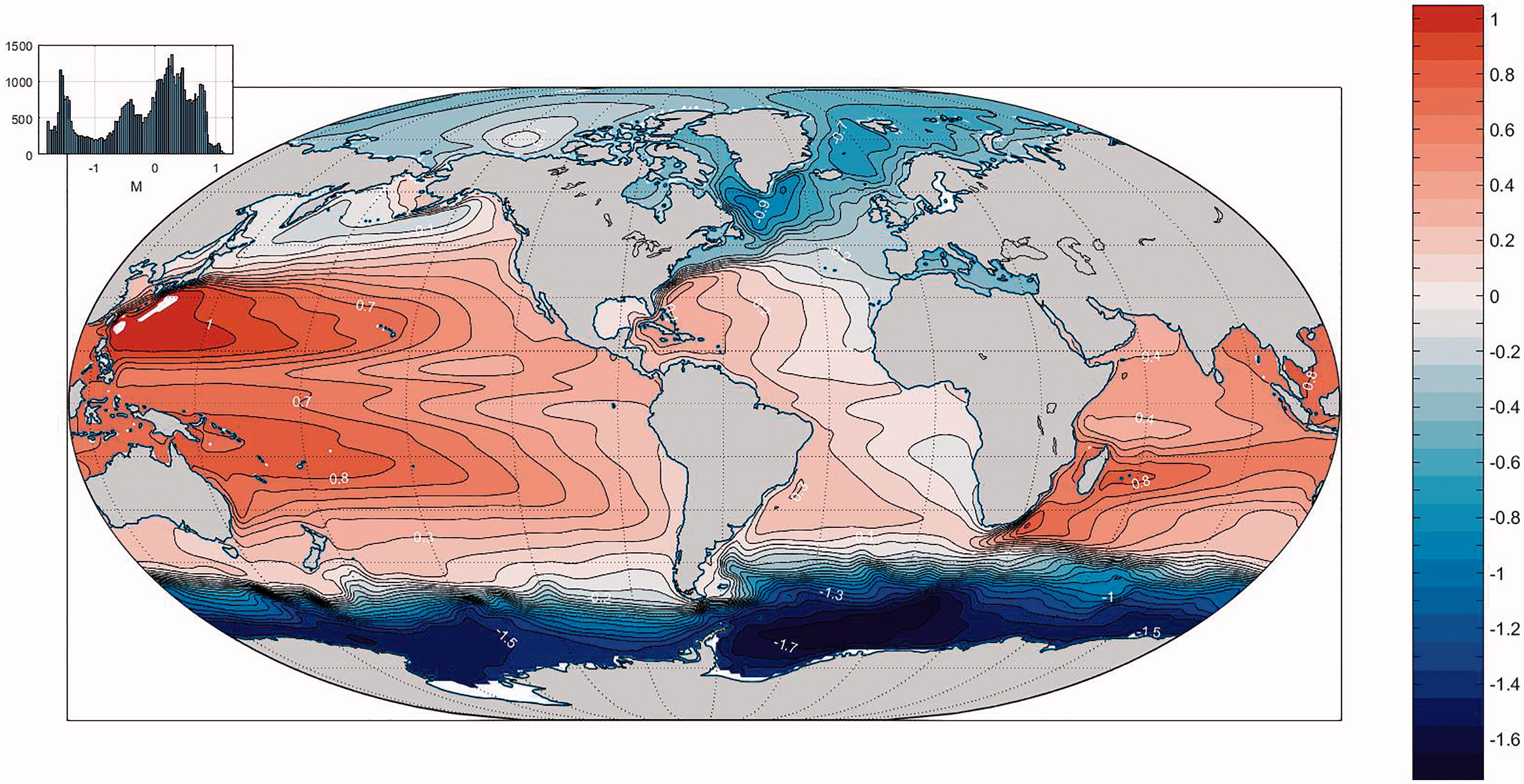
Fig. 5.
Time mean elevation (dynamic height) corrected for ice cover weight (Fukumori et al. 2018). Values are multimodal.
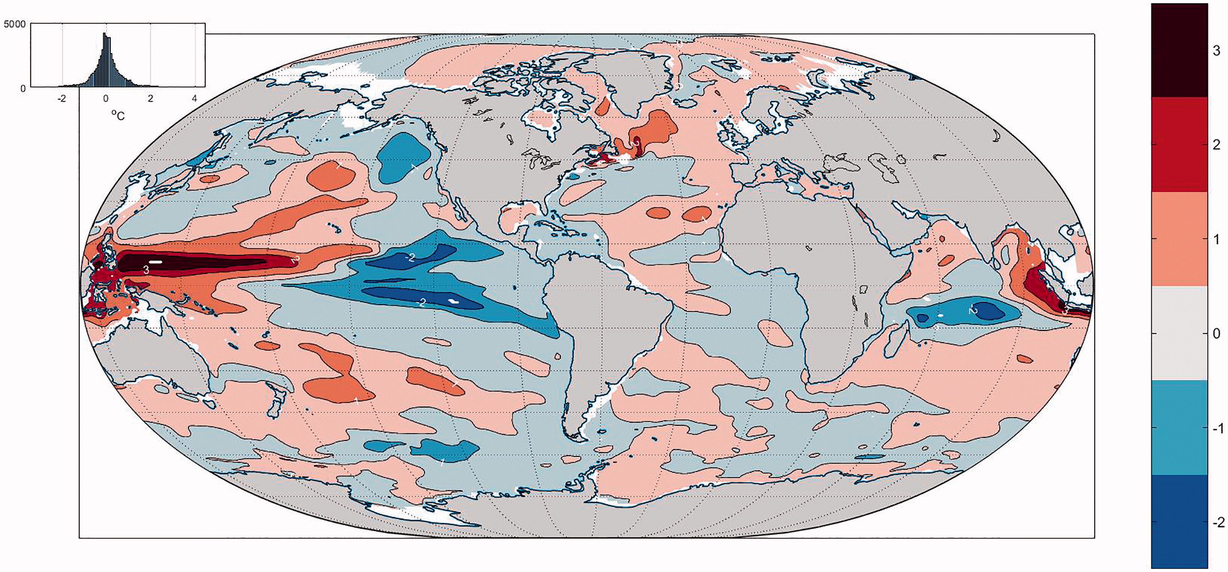
Fig. 6.
Temperature difference at 105 m between 2013 and 1994 (°C). Values are unimodal.
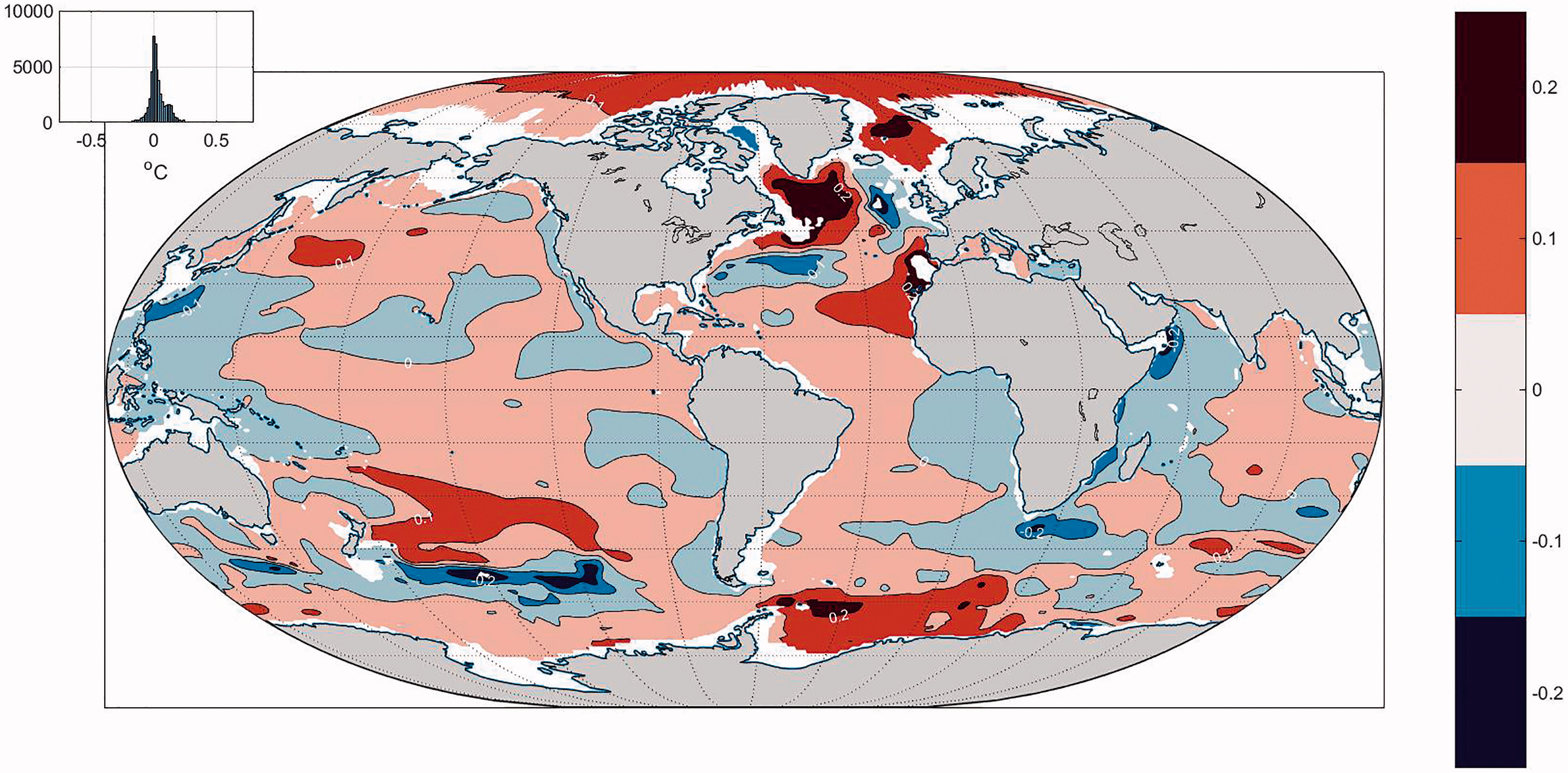
Fig. 7.
Temperature difference (oC) at 1000 m between 2013 and 1994.
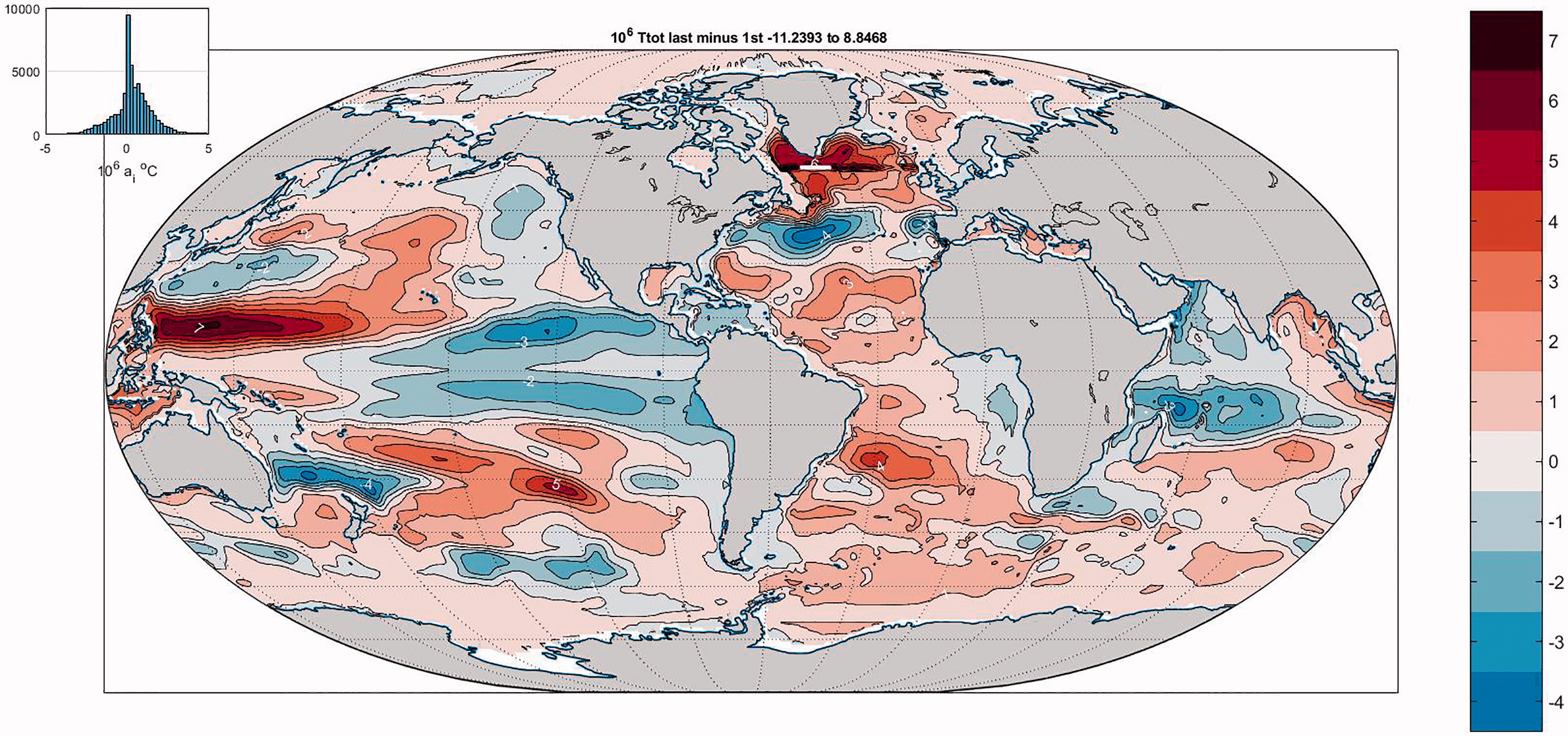
Fig. 8.
Vertical integral, top-to-bottom, of the temperature difference between 2014 and 1993 and area weighted (106 °C). The result is treated as fully stochastic, which may somewhat overestimate the formal uncertainty (. Histogram is again unimodal. Spatial complexity here is indicative of the difficult oceanic sampling problem.
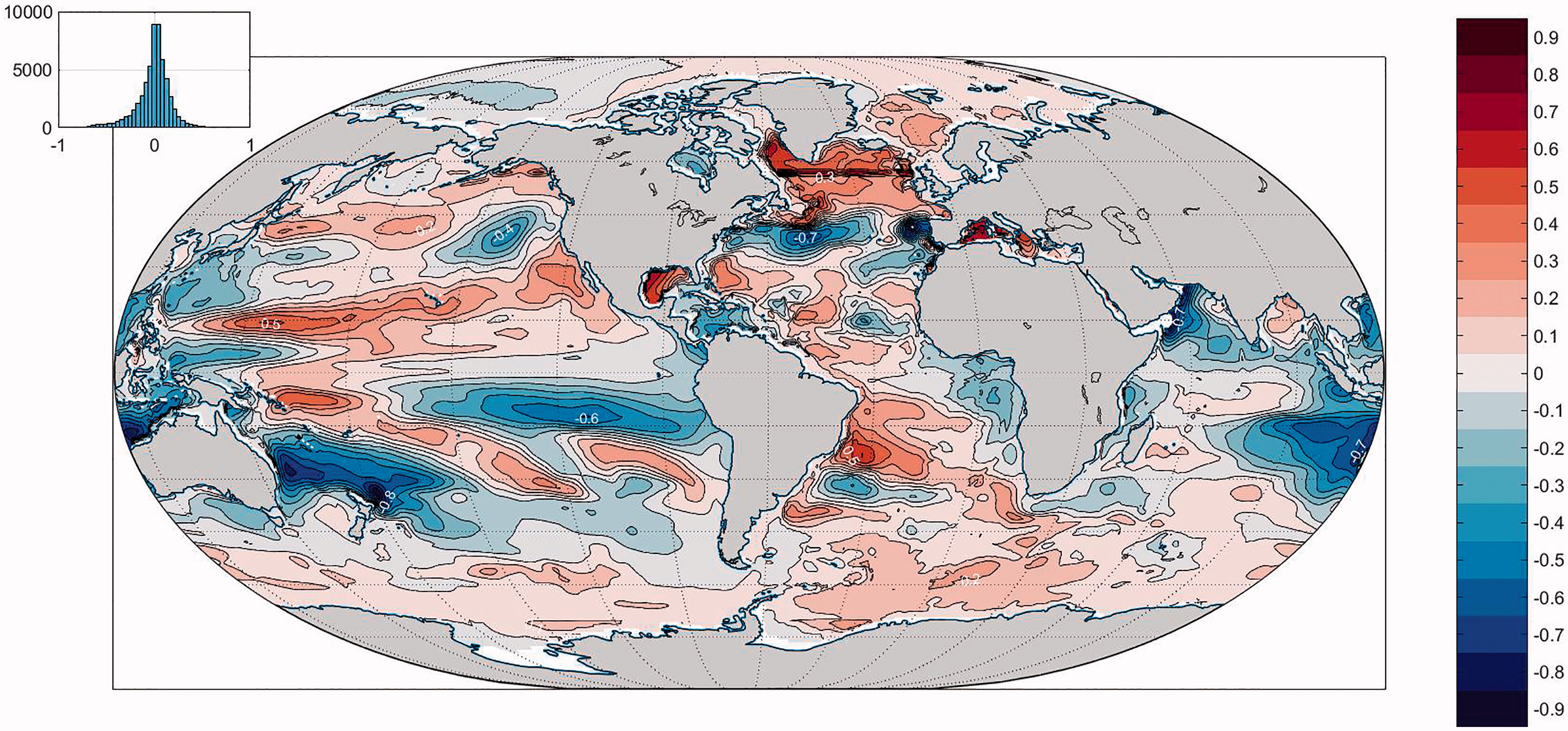
Fig. 9.
Vertically integrated salinity difference 2013–1994, top-to-bottom.
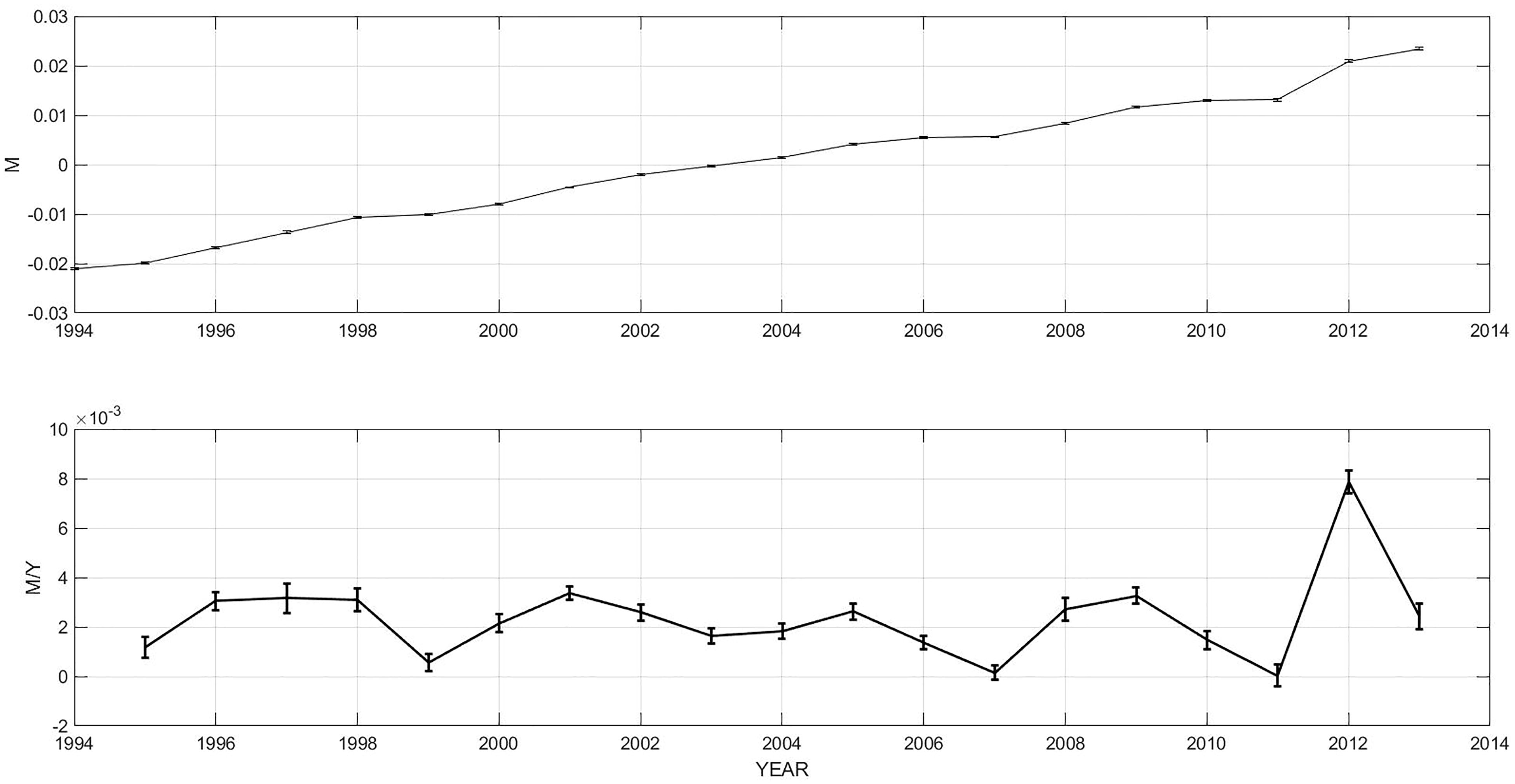
Fig. 10.
Annual mean anomaly of surface elevation (m) relative to the 20-year mean in Fig. 5 over 20 years (upper panel). Error estimates are from a bootstrap of the spatial distribution of the anomaly field in each year, with q = 0. Lower panel shows the simple year-to-year difference of the values in the upper panel with the uncertainty estimates between each year treated as independent.
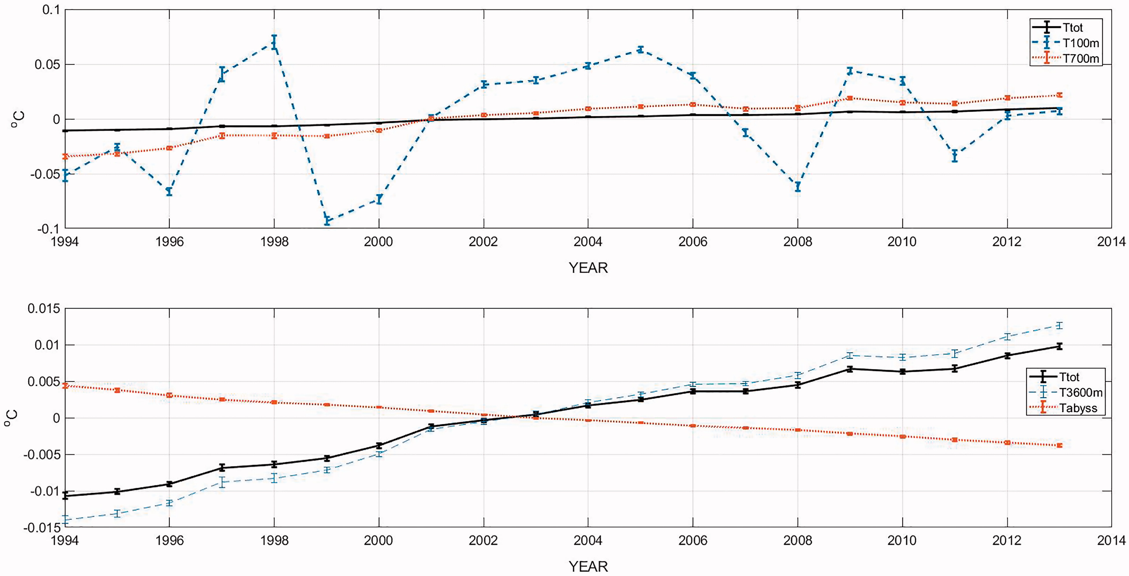
Fig. 11.
Annual mean temperature anomalies integrated to different depths including the bottom in °C. Two standard deviation bars are derived from bootstrapping the full temperature difference field each year. Ttot is integrated top-to-bottom; T100m, T700m, T3600m are integrated to 100, 700, and 3600 m, respectively. Tabyss is integrated from 3600 m to the bottom. Cooling in the region below 3600 m was discussed by Wunsch and Heimbach (2014) and Gebbie and Huybers (2018).
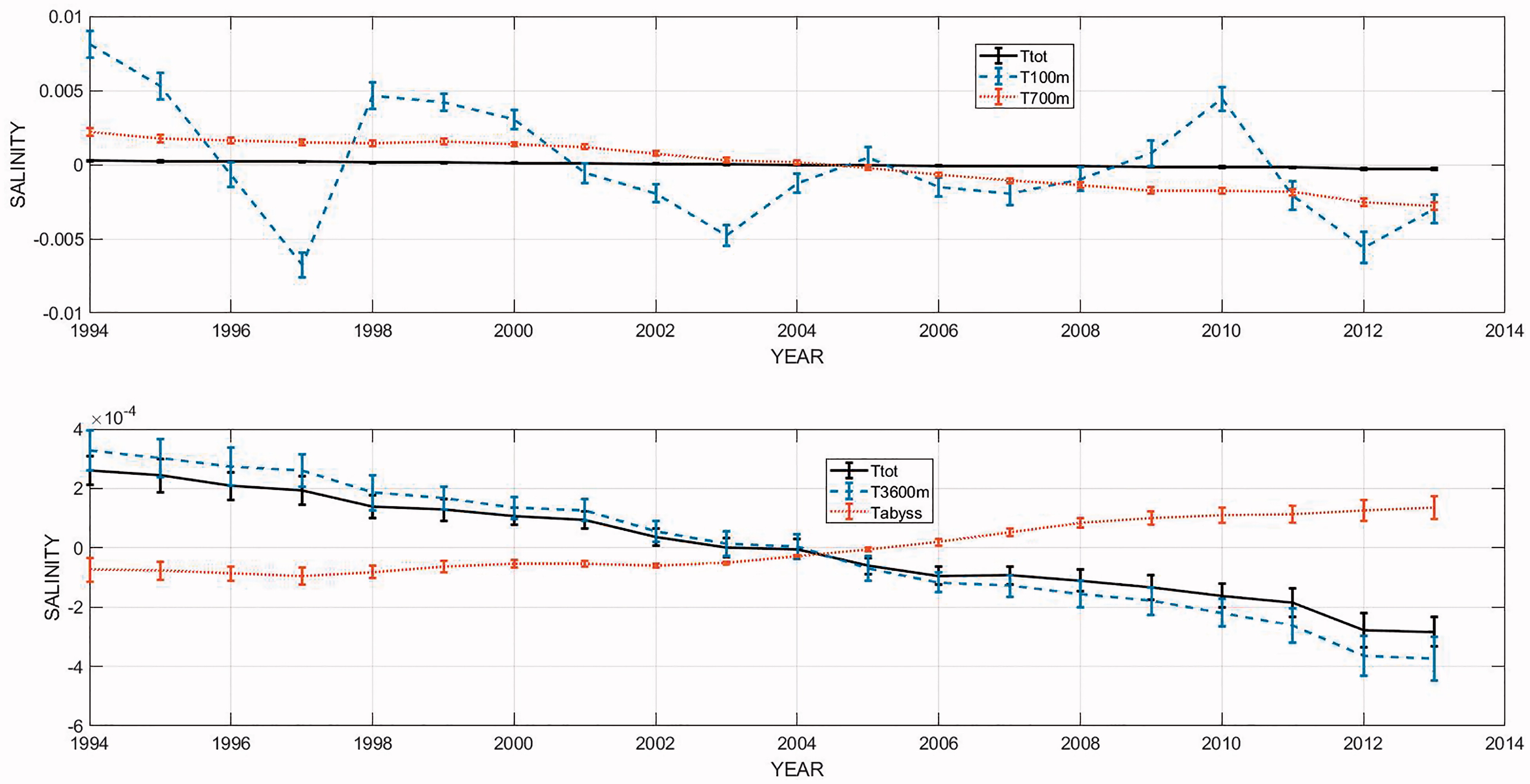
Fig. 12.
Same as Fig. 9, except for the mean vertically integrated salinity anomaly (practical scale) for each year with an estimated 2-standard deviation error bar. Total is repeated in both panels. Note overall freshening, with a partly compensating increase in salinity in the abyss. A best-fitting linear trend for the total change is discussed in the text.