
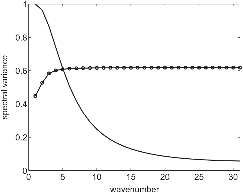
Figure 1.
Spectral variances of the Kalman gain matrix for a fully observed system. Line with markers is the case where the length scale of observation error correlations is greater than that of the background error correlations; solid line is for the case where the length scale of the background error correlations is greater than that of the observation error correlations.
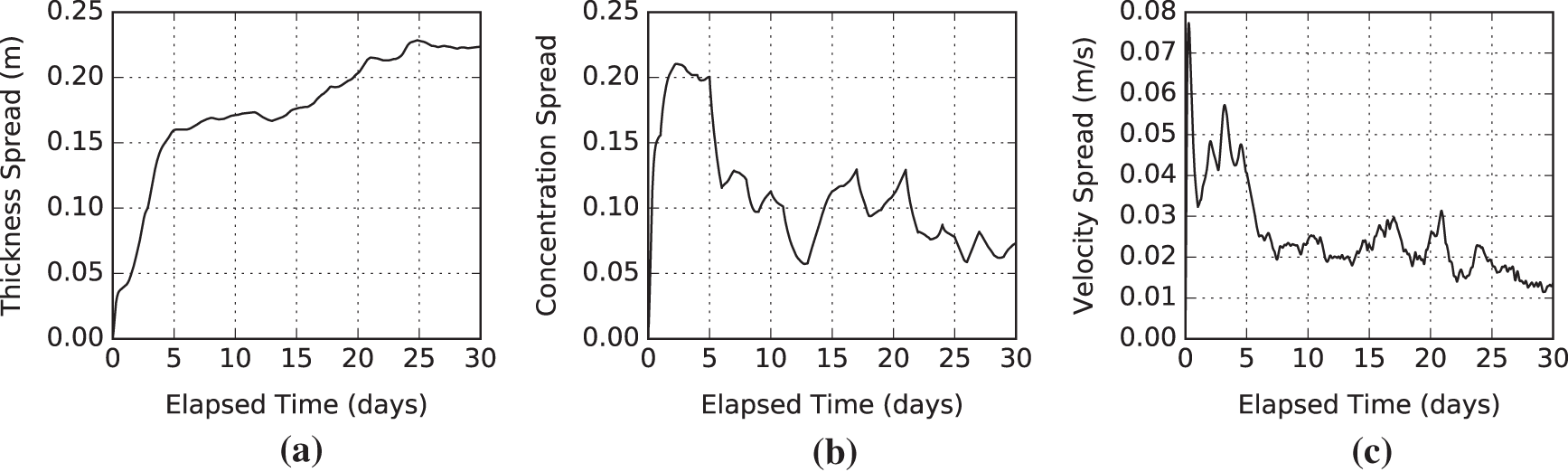
Figure 2.
Temporal evolution of spread in the five-hundred-member ensemble during the thirty-day freeze-up period. The thickness spread (a) increased gradually to a value of approximately 0.23 m. The concentration (b) and velocity (c) spreads increased abruptly at the beginning of the simulation, but gradually decreased as the mean concentration approached 100% and the ice strengthened.
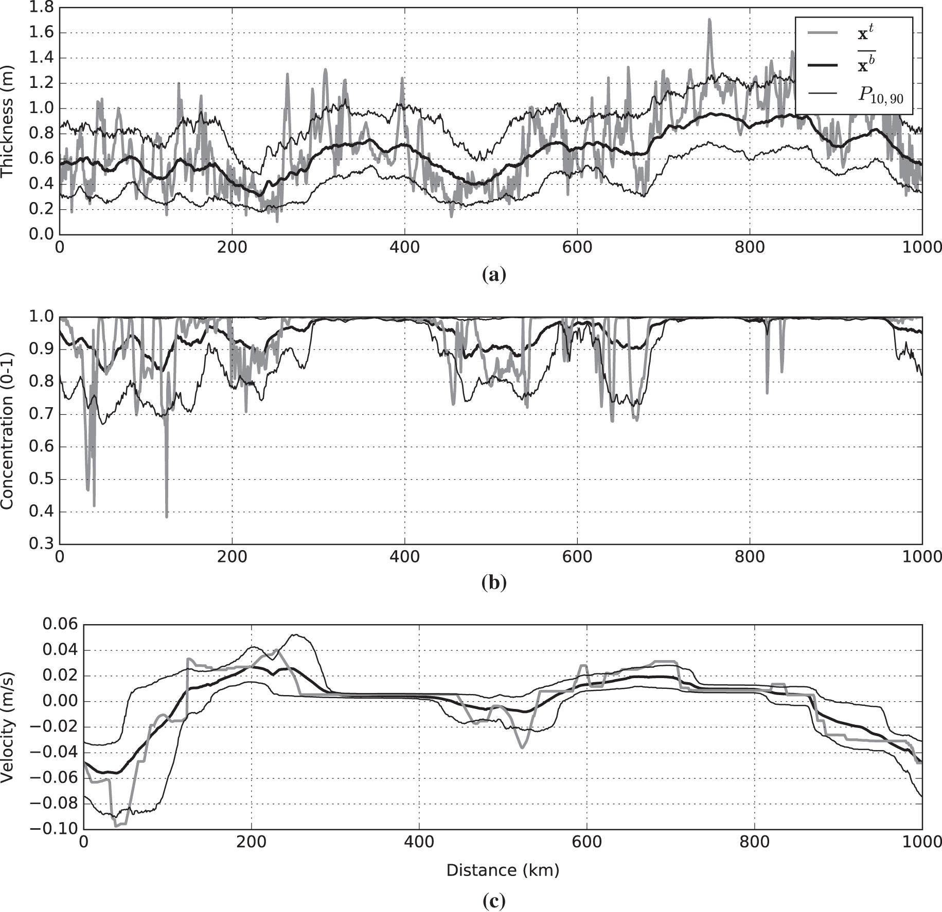
Figure 3.
Ensemble of sea ice model states with the true state following the thirty-day freeze-up period. The mean and the 10th/90th percentiles of the ensemble are plotted to illustrate the spread. Note that where the true ice concentration was near 100%, the spread of the ice concentration and the velocity errors were the least but there was little correlation between the state and the thickness spread.
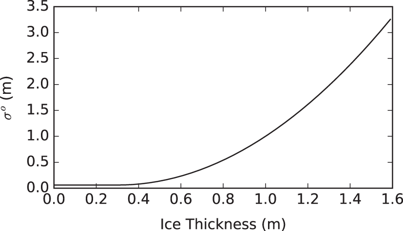
Figure 4.
Prescribed true observation error standard deviation as a function of ice thickness. As the true ice thickness increases beyond 0.3m, the observation error standard deviation increases quadratically, meaning that there is low observation accuracy for regions of thick i.e.
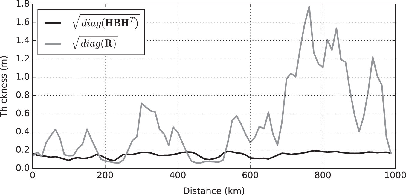
Figure 5.
Evaluation of the ice thickness observation error standard deviation function at the true state mapped to the observation locations. The background error standard deviations (solid black) can be compared to the observation error standard deviations (grey), revealing that the background error standard deviations are relatively constant across the domain while the observation error standard deviations are more variable. We can expect greater impact from the assimilation in two isolated regions where the observation error standard deviations are less than the background error standard deviations.
Table 1.
Correlation structure of each observation error covariance matrix.
Table 2.
Four variants of the analysis error covariance matrix that were computed for each twin experiment.
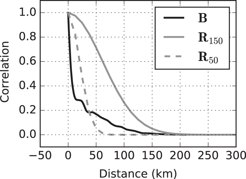
Figure 6.
Correlation structure of ice thickness errors extracted from the background error covariance matrix compared to the prescribed error correlation structures for the observation error covariance matrices.
Table 3.
Analysis error standard deviations for ice thickness (h), ice concentration (a) and ice velocity (u) for the case where (left column), (centre column), and (right column).
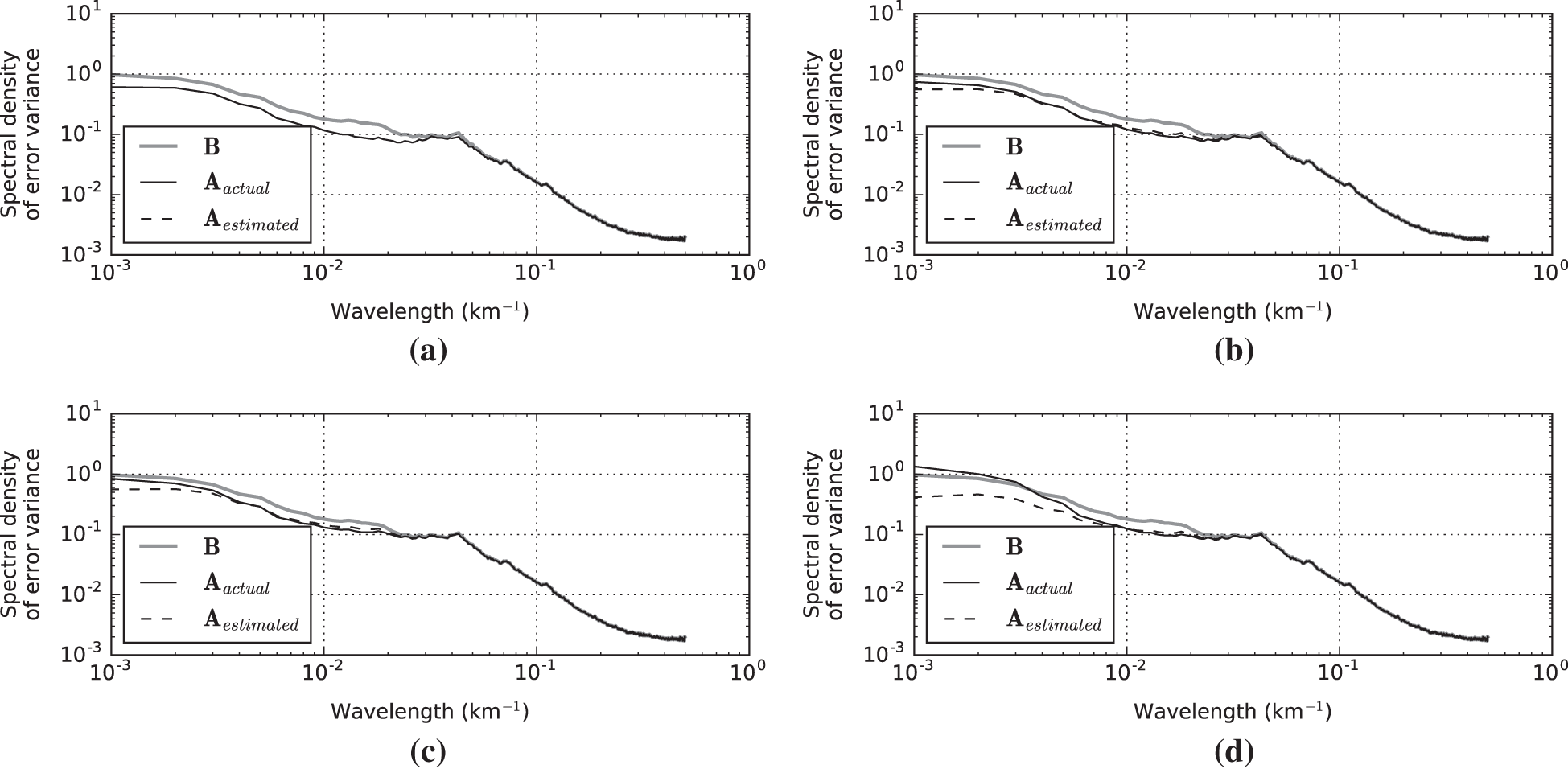
Figure 7.
Spectral densities of thickness analysis error variances for the experiment where the true observation error covariance matrix had an exponential correlation structure with decorrelation length of 150 km. Panel (a) , (b) , (c) , (d) .
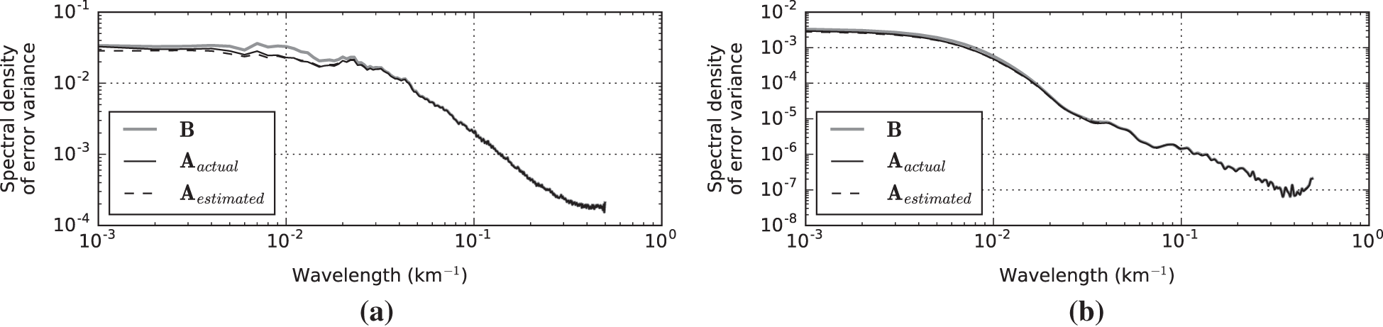
Figure 8.
Spectral densities of (a) ice concentration and (b) ice velocity, analysis error variances for the experiment where and .
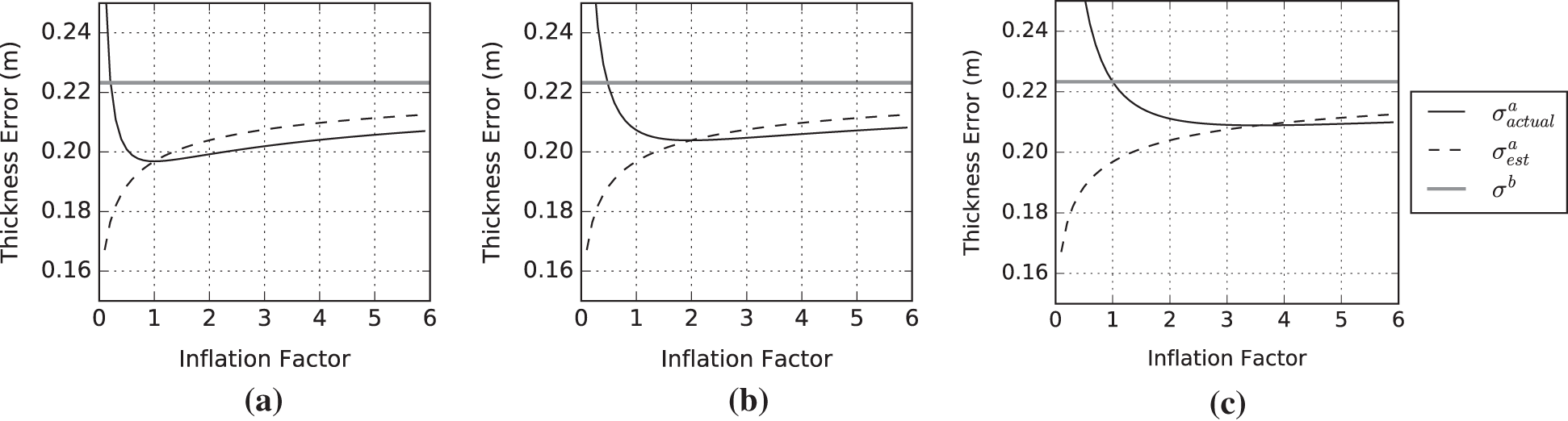
Figure 9.
Estimated and actual thickness analysis error standard deviation as a function of the inflation factor for (a) (b) and (c) . Each experiment had an optimal inflation factor between 1 and 4. Underestimation of the inflation factor resulted in a divergence between the estimated and actual analysis error standard deviation. Overestimation of the inflation factor had a lesser effect.