
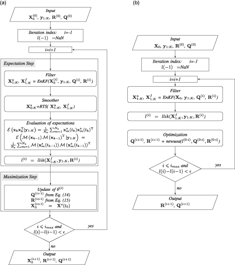
Figure 1.
(a) Flowchart of the EM algorithm (left panel). (b) NR flowchart (right panel). Each column of the matrix is an ensemble member state at time k. Subscript (i) means ith iteration. A final application of the filter may be required to obtain the updated analysis state at . The function llik is the log-likelihood calculation from (21). The newuoa function in the optimization step refers to the ’new’ unconstrained optimization algorithm (Powell, 2006).
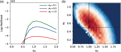
Figure 2.
Log-likelihood function as a function of (a) model noise for three true observational noise values, ; and as a function of (b) model noise () and observational noise () for a case with and . Darker red shading represents larger log-likelihood.
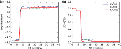
Figure 3.
Convergence of the NR maximization as a function of the iteration of the outer loop (inner loops are composed of function evaluations, where is the control space dimension) for different evidencing window lengths (). (a) Log-likelihood function. (b) Frobenius norm of the model noise estimation error.
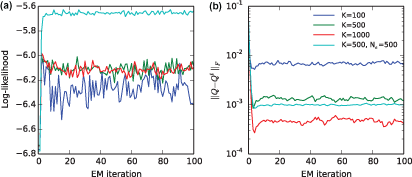
Figure 4.
Convergence of the EM algorithm as a function of the iteration for different observation time lengths (evidencing window). An experiment with ensemble members and is also shown. (a) Log-likelihood function. (b) The Frobenius norm of the model noise estimation error.
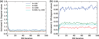
Figure 5.
Estimated model noise as a function of the iteration in the EM algorithm. (a) Mean diagonal model noise (true value is 1.0). (b) Mean off-diagonal absolute model noise value (true value is 0.0).
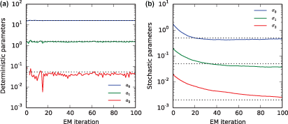
Figure 6.
(a) Estimated mean deterministic parameters, , as a function of the EM iterations for the twin parameter experiment. (b) Estimated stochastic parameters, .
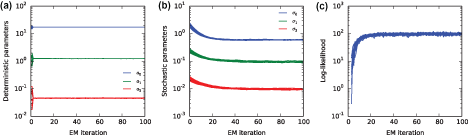
Figure 7.
(a) Estimated deterministic parameters as a function of the EM iterations for the model-identification experiment. Twenty experiments with random initial deterministic and stochastic parameters are shown. (b) Estimated stochastic parameters. (c) Log-likelihood function.
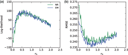
Figure 8.
(a) Log-likelihood as a function of the parameter at the and optimal values for the NR estimation (green curve) and with the optimal values for the EM estimation (blue curve) for the imperfect-model experiment. (b) Analysis RMSE as a function of the parameter.
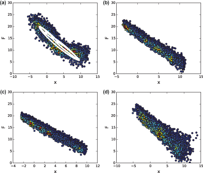
Figure 9.
(a) Scatterplot of the true small-scale effects in the two-scale Lorenz-96 model as a function of a large-scale variable (coloured dots) and scatterplot of the deterministic parameterization with optimal parameters (white dots). (b) Scatterplot from the stochastic paramerization with optimal parameters obtained with the EM algorithm and (c) with the NR method. (d) Scatterplot given by a constrained random walk with optimal EM parameters.