Have a personal or library account? Click to login
Modified parameterization of the vertical water temperature profile in the FLake model Cover

Modified parameterization of the vertical water temperature profile in the FLake model

Open Access
|Jan 2018

Figures & Tables

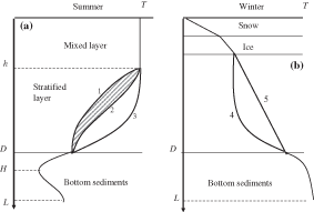
Fig. 1.

The scheme of the vertical temperature distribution in the system ‘snow – ice – water – bottom sediments’ realized in the model FLake: (a) open water case; (b) ice-covered period.

Table 1.

Parameterizations suggested by different authors to describe the vertical distribution of temperature in water basins.
AuthorsParameterizationApplicationAnderson and Munk 1947 (cited from Mironov 2008)Verbal mention of the ‘almost constant shape’ of the temperature profile beneath the upper mixed layerLake water columnKitaigorodskii and Miropolsky (1970)T(ζ)=83·ζ-2·ζ2+13·ζ4(8)Oceanic active layer Arsenyev and Felzenbaum (1977)T*(ζ) = 1 – (1 – ζ)3(9)Oceanic active layerMalkki and Tamsalu (1985)T(ζ)=1-(1-ζ)3atdh/dt>01-4·(1-ζ)3+3·(1-ζ)4atdh/dt0(10)Baltic Sea active layer, water column of lakesGolosov et al. (2003)T*(ζ) = (2 – B(t)) ⋅ ζ + (B(t) – 1) ⋅ ζ2(11)Water column of lakes at ice cover periodMironov (2008)T*(ζ) = ζ(12)Water column of lakes at ice cover period, snow and ice cover Golosov et al. (1998); Golosov and Kirillin (2010)T1(ξ1)=2·ξ1-ξ12atDzHT2(ξ2)=3·ξ22-2·ξ23atHzL(13)Bottom sediments of lakes
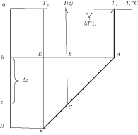
Fig. 2.

The scheme of linear temperature profile (Table of symbols in Fig. 2 are the same as those in Fig. 1), T(z) is temperature at depth z, A, B, C, D, E are the vertices of a right triangles.
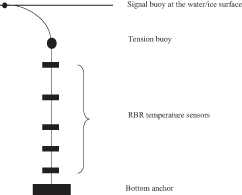
Fig. 3.

Allocation scheme of temperature sensors at the thermistor chain.
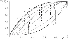
Fig. 4.

Relationship between different parameterizations. Here empty circles mark ‘winter’ data, black squares stand for data, obtained during the open water period; upper solid line coincides with parameterization (16) at A = 3 and B = 0, the lower solid line coincides a new parameterization (16) at A = 0 and B = 3. Intermediate thin lines correspond to parameterizations (8)–(13).

Table 2.

Relationship between different parameterizations.

AuthorsParameterizationValues of A(t) and B(t) in new parameterizationKitaigorodskii and Miropolsky (1970)T(ζ)=83·ζ-2·ζ2+13·ζ4(8)A=2.85B=0Arsenyev and Felzenbaum (1977)T*(ζ) = 1 – (1 – ζ)3(9)A=3,B=0Malkki and Tamsalu (1985)T(ζ)=1-(1-ζ)3atdh/dt>01-4·(1-ζ)3+3·(1-ζ)4atdh/dt0(10)A=3,B=0A=?,B=?Golosov et al. (2003)T*(ζ) = (2 - B(t)) ⋅ ζ + (B(t) – 1) ⋅ ζ2(11)A(t) ∊ [0, 2], B(t) ∊ [0, 2]Mironov (2008)T*(ζ) = ζ(12)A = 1, B = 1Golosov et al. (1998); Golosov and Kirillin (2010)T1(ξ1)=2·ξ1-ξ12atDzHT2(ξ2)=3·ξ22-2·ξ23atHzL(13)A=2,B=0A=0,B=0
Language: English
Page range: 1441247 - 1441247
Submitted on: Mar 25, 2017
Accepted on: Feb 1, 2018
Published on: Jan 1, 2018
Published by: Stockholm University Press
In partnership with: Paradigm Publishing Services

© 2018 Sergey Golosov, Ilia Zverev, Ekaterina Shipunova, Arkady Terzhevik, published by Stockholm University Press
This work is licensed under the Creative Commons Attribution 4.0 License.