
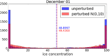
Figure 1.
Histogram of the synthetic observations of sea ice concentration (aice [%]) in December 1 without added white noise (blue) and with added white noise (red) with 10% standard deviation and cut-off of unphysical values. The evaluation is restricted to grid cells in which TRUTH contained sea ice at least once. The dashed lines indicate the mean values of the resulting ice concentrations, which differ between the unperturbed and the perturbed case.
Table 1.
List of experiments analysed. The second and the third column detail the variables assimilated in the sea ice and in the ocean. The right column indicates the variables that are diagnosed a posteriori, see also Appendix, Table A1. The index ‘1 : 5’ refers to the five thickness categories, while the lack of an index in the ice state variables refers to the aggregate values. The abbreviation ‘ML’ refers to the elements in the mixed layer of the ocean, i.e. layers 1 and 2; ‘:’ indicates that we include the entire ocean column into the state vector.
Table 2.
List of variables. We use the five thickness categories of CICE4.0 with one being the thinnest and five the thickest.
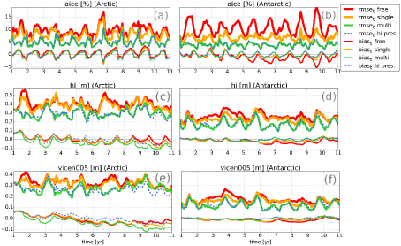
Figure 2.
(bold lines) and (thin lines) of aice (a,b), hi (c,d) and vice (e,f) in the Arctic (left column) and in the Antarctic (right column) for FREE (red), SINGLE (orange), MULTI (green) and HI_PRESERVE (blue).
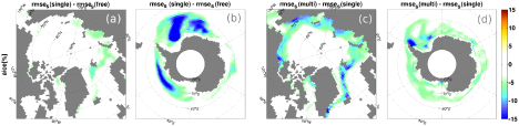
Figure 3.
Differences in of aice between SINGLE and FREE in the Arctic (a) and in the Antarctic (b) with maximum of 29%, and between MULTI and SINGLE in the Arctic (c) and in the Antarctic (d) with maximum of 21%.
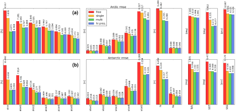
Figure 4.
rmse of all considered variables for FREE (red), SINGLE (orange), MULTI (green) and HI_PRESERVE (blue) restricted to the Arctic region (a) and to the Antarctic region (b), respectively.
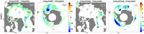
Figure 5.
Differences in of aice between WEAK and FREE in the Arctic (a) and in the Antarctic (b) with maximum of 35%, and between STRONG and WEAK in the Arctic (c) and in the Antarctic (d) with maximum of 14%.
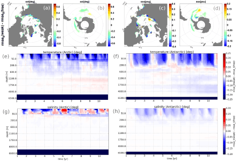
Figure 6.
Differences in between WEAK and FREE for SST in the Arctic (a) and in the Antarctic (b), for SSS in the Arctic (c) and in the Antarctic (d). Cool colours indicate an improvement, warm colours a degradation in WEAK compared to FREE. Panels (e,f) and (g,h) depict the differences in in temperature and salinity in the Arctic and in the Antarctic for different depths between WEAK and FREE with latitudes .
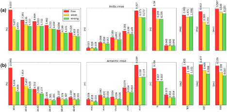
Figure 7.
Time and space averaged rmses of the ice component and of the 2D sea surface salinity and temperature for FREE (red), WEAK (yellow) and STRONG (green) in the Arctic (a) and the Antarctic (b).
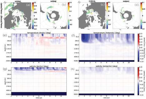
Figure 8.
Differences in between STRONG and WEAK for SST in the Arctic (a) and in the Antarctic (b), for SSS in the Arctic (c) and in the Antarctic (d). Cold colours indicate an improvement and warm colours a degradation of STRONG compared to WEAK. Panels (e,f) and (g,h) depict the differences in in temperature and salinity for different depths between STRONG and WEAK for latitudes in the Arctic and in the Antarctic, respectively.
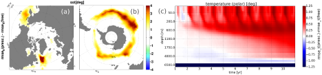
Figure 9.
Panels (a) and (b): differences of the values of SST of PRESCRIBED and FREE for the Arctic and the Antarctic region. Panel (c): Hovmöller diagram for the differences in of the temperature field of PRESCRIBED and FREE restricted to regions with latitudes .
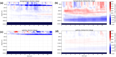
Figure 10.
Hovmöller diagrams for the differences in of the temperature field (a,b) and the salinity field (c,d) between DEPTH and STRONG, restricted to regions with latitudes in the Arctic and in the Antarctic, respectively.
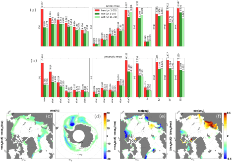
Figure 11.
Panel (a) and (b) depict the time and space averaged rmses of the ice component and of the 2D SST and SSS for FREE (red), the optimal run in the first decade (green) and the optimal run in the second decade (light green) in the Arctic and in the Antarctic. Panels (c) and (d) show differences in for aice between the optimal run and the free run averaged over the first 10 years; panel (e) shows the differences in for SSS and panel (f) in for the first 10 years.
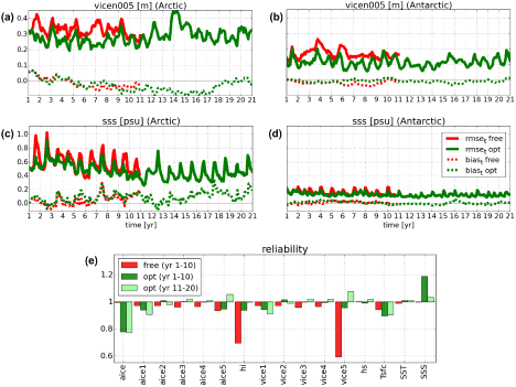
Figure 12.
Panels (a,b) and (c,d): (bold lines) and (dotted lines) of vice and SSS for FREE (red, only first 10 years) and for the optimal setting (green, 20 years) in the Arctic and in the Antarctic, respectively. Panel (e) shows the summary of the global time and space averaged reliabilities of all considered variables for FREE (red), and the optimal setting (green), where the evaluation is splitted into decades.
Table A1.
List of postprocessings (upper part) and diagnosed variables (lower part, see Table 2 for an explanation of the variables). Variables with index f are forecast values, those with index a are the values after the analysis and variables with index p denote values after the postprocessing. The index pp denotes a second postprocessing of the already postprocessed variable. and denote the lower and the upper bound of the n-th thickness category (predefined CICE4.0 values). is the threshold, set to . ML refers to the ocean mixed layer. SINGLE, HI_PRESERVE, DEPTH HI_PRESERVE and PRESCRIBED are particular experiments differing in the assimilation state vector and the diagnosed variables. The general case applies for all of the considered experiments, see also Table 1 for an overview.