
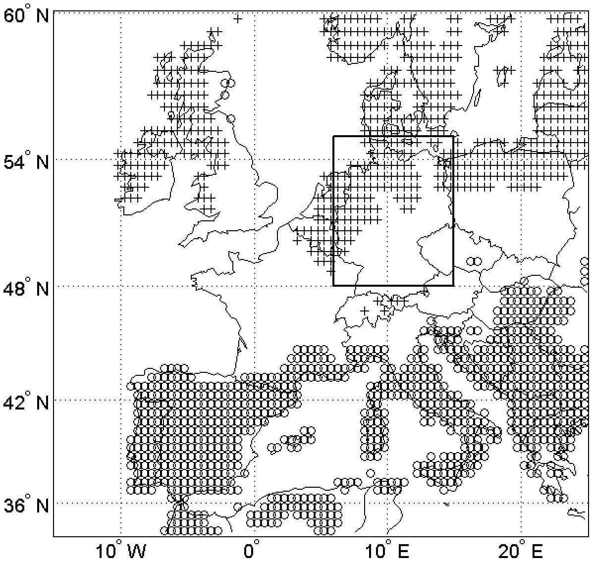
Fig. 1.
Correlation map of DJFM precipitation with NAO at 5% significance level for the period from 1981 to 2014.
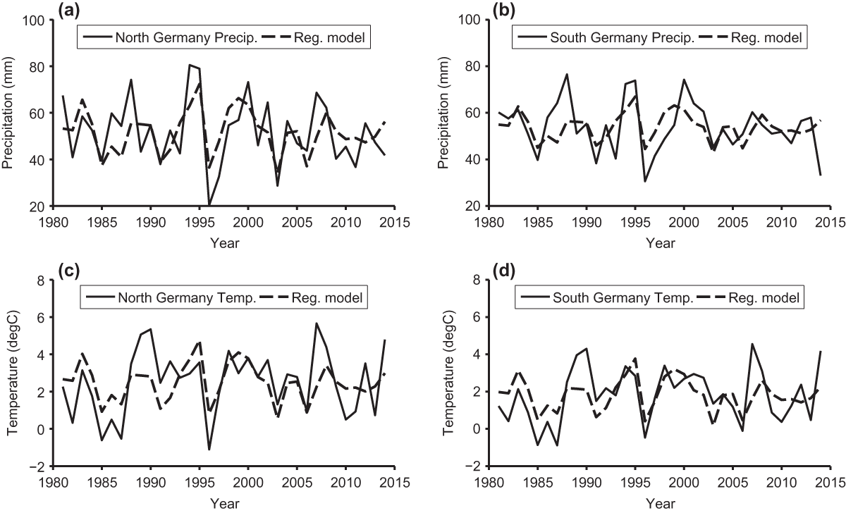
Fig. 2.
Time series comparison between (a) observed precipitation over north Germany and the regression model, (b) observed precipitation over south Germany and the regression model, (c) observed temperature over north Germany and the regression model and (d) observed temperature over south Germany and the regression model. In the regression models ILLN is taken as independent variable.
Table 1.
Data used, its sources and latitude/longitude resolution.
Table 2a.
Correlation coefficients between precipitation of Northern and Southern Germany and COA indices and NAO.
Table 2b.
Correlation coefficients between mean temperature of Northern and Southern Germany and COA indices and NAO.
Table 3.
Partial correlation between DJFM rainfall of northern Germany and the given variable by controlling all the other variables. The five independent variables considered here are AZH pressure, AZH longitude, IL latitude, IL longitude and NAO.
Table 4.
Partial correlation between DJFM mean temperature of northern Germany and the given variable by controlling all the other variables. The seven independent variables considered here are AZH pressure, AZH latitude, IL pressure, IL latitude, IL longitude and NAO.
Table 5.
Partial correlation coefficients between mean DJFM temperature of Southern Germany with a given variable. The five independent variables considered here are AZH pressure, IL pressure, IL latitude, IL longitude and NAO.
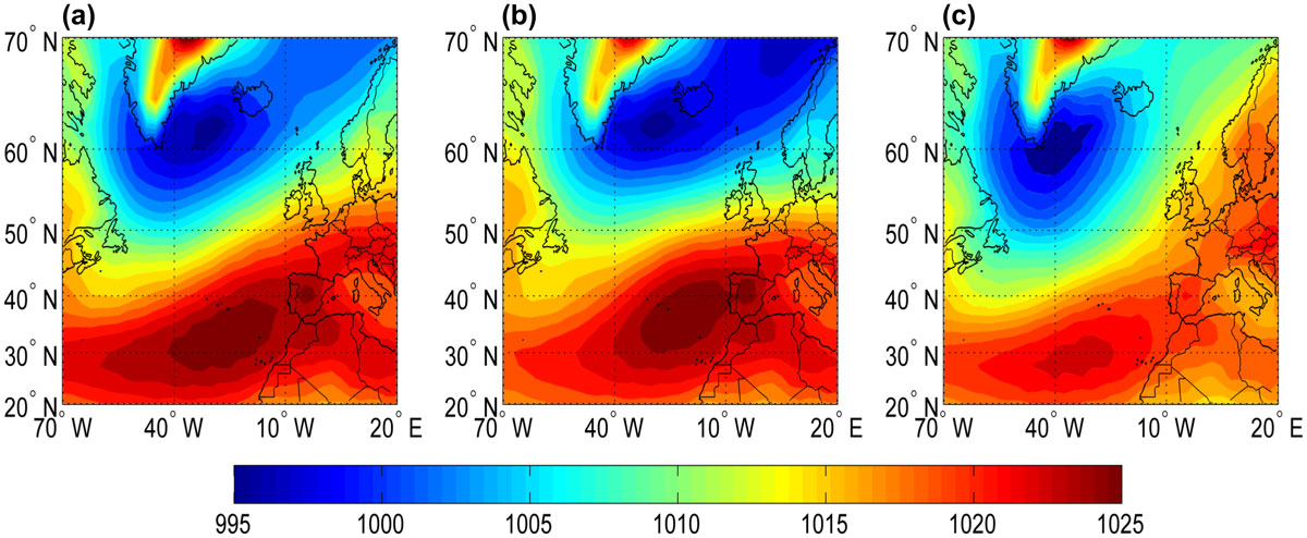
Fig. 3.
Sea level distribution over north Atlantic (a) averaged for 1981–2014, (b) when Icelandic Low is situated to the east of its mean location by more than one standard deviation and (c) when Icelandic Low is situated to the west of its mean location by more than one standard deviation.
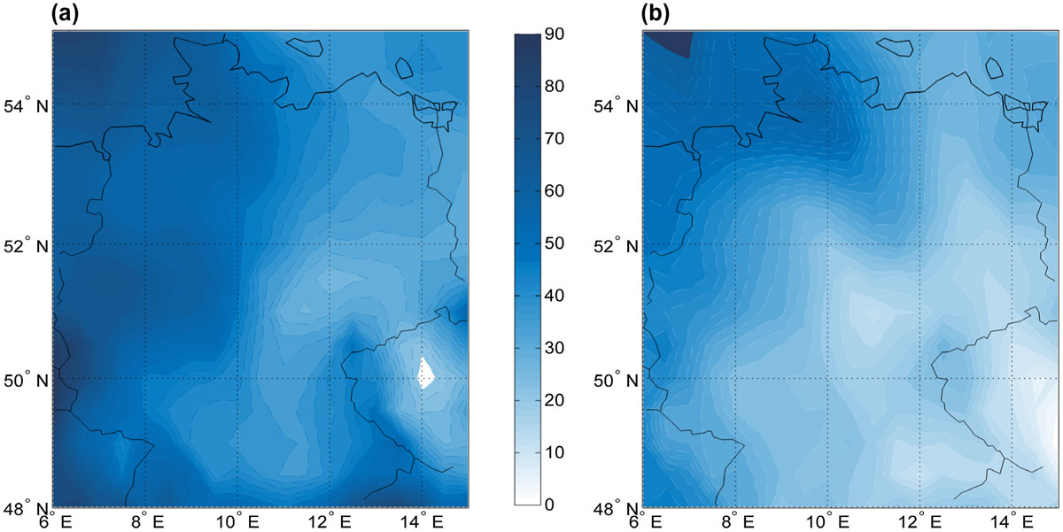
Fig. 4.
(a) Climatological mean of Germany precipitation (in mm) from 1981 to 2010 and (b) difference of mean precipitation between IL E and IL W winters.

Fig. 5.
(a) Climatological mean of DJFM air temperature (°C) from 1981 to 2010 and (b) difference of mean air temperature between IL E and IL W winters.
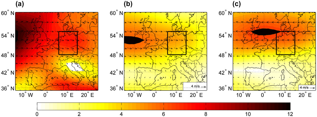
Fig. 6.
(a) Mean wind over western Europe at 700 mb height (1981–2010), (b) composite anomaly map for vector wind at 700 mb level when Icelandic Low longitude is east of its mean value by one standard deviation and (c) composite anomaly map for vector wind at 700 mb level when Icelandic Low longitude is west of its mean value by more than one standard deviation. Shading corresponds to the wind speed.
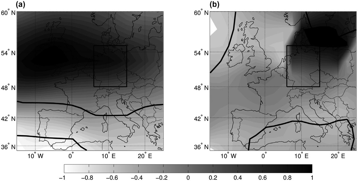
Fig. 7.
(a) Difference in wind speeds for IL E years and IL W years and (b) difference in angles at each grid point for IL E years and IL W years. Solid black line indicates the grid points where the angles are different at p < 0.05 level.
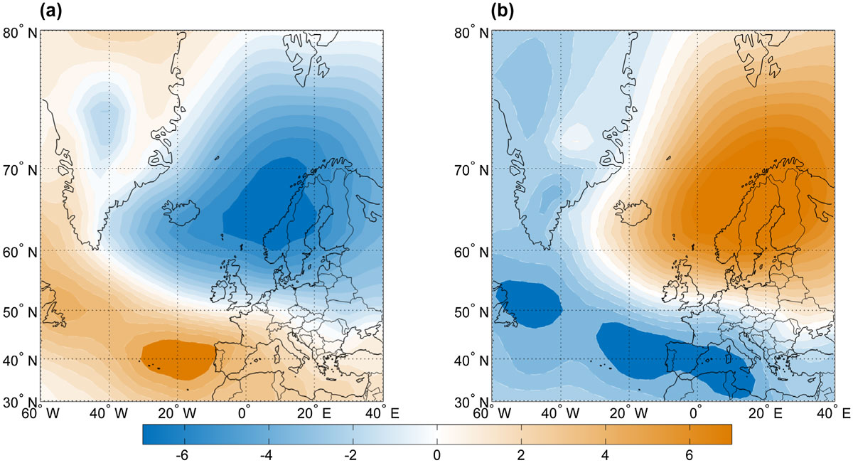
Fig. 8.
(a) Composite anomaly map for SLP in winters when the Icelandic Low is situated east of its mean longitude position by more than one standard deviation and (b) composite anomaly map for SLP in winters when the Icelandic Low is situated west of its mean longitude position by more than one standard deviation.

Fig. 9.
Student’s t-test for difference in SLP at each grid point for IL E years and IL W years. Solid black line indicates the grid points where the angles are different at p < 0.05 level.