
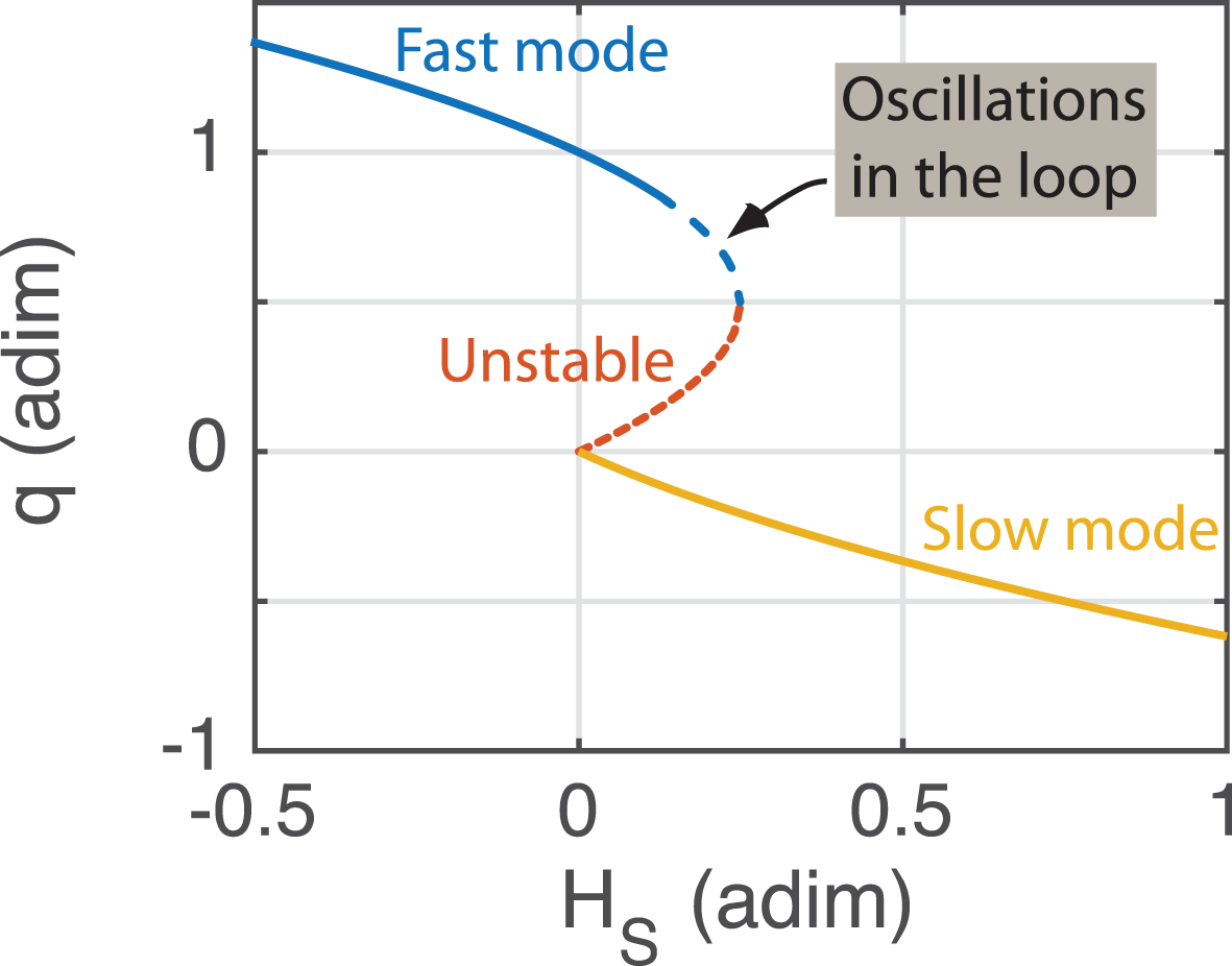
Figure 1.
Steady-state solutions of a Stommel two-box model, showing a range of bi-stability between a temperature-controlled fast mode (blue) and a salinity-controlled slow mode (yellow). The intermediate state (red) is unstable. In this study, we will show that in the thermohaline loop model, the fast mode becomes subject to an oscillatory instability before the turning point, effectively reducing the range of bi-stability.
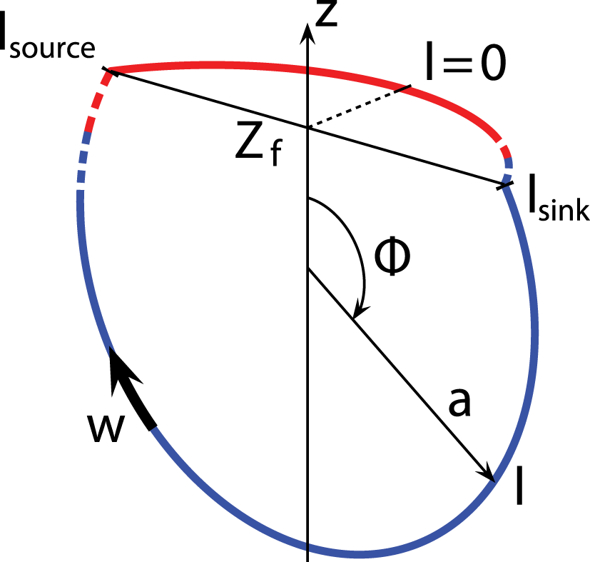
Figure 2.
Schematics of the folded loop configuration. Adapted from Pollmann et al. (2015).
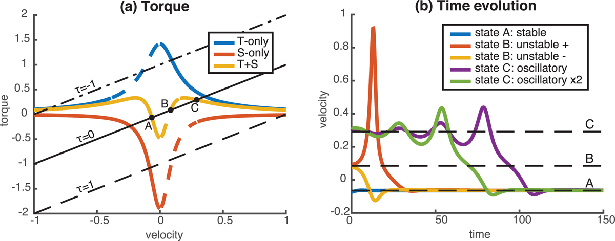
Figure 3.
(a) Torque curves for Case 1 (see Table 1). The buoyancy torque curve is plotted for a temperature-only (blue curve, T-only), salinity-only (red curve, S-only) or both forcings together (yellow curve, T+S). Possible steady states are determined as the intersection between the buoyancy torque curve and the frictional minus applied torque line. Dashed lines denote unstable regions, where . Multiple equilibria can be found for the three cases when a suitable torque is applied. For example, for the mixed case with no applied torque (yellow curve intersecting the solid black line), three steady states, denoted A, B and C, are found. (b) Time evolution of the loop velocity for the three steady states A, B and C of the no-applied-torque mixed case T+S, following a small perturbation. A perturbation of 0.01 in velocity is applied around steady states, except for the ‘oscillatory x2’ case where a 0.02 velocity perturbation is applied instead.
Table 1.
Parameter list of study cases. Case 1 is used as the reference case throughout this study. Other cases are mainly discussed in section 4c (see Fig. 6).
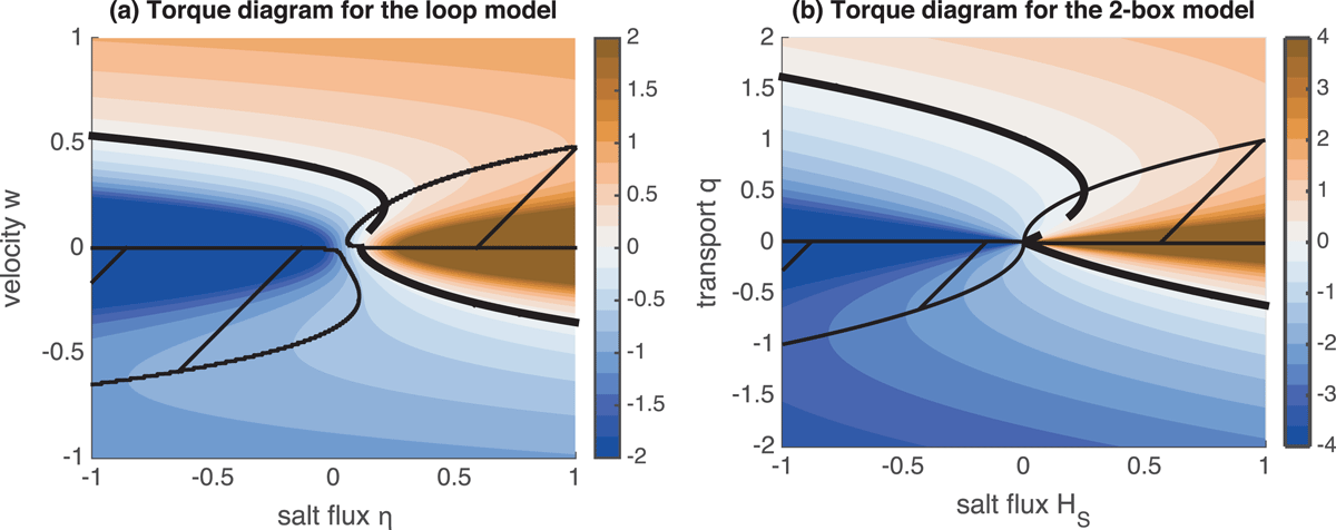
Figure 4.
(a) Torque diagram for Case 1. Colour contours correspond to the torque that must be applied to achieve a steady state, shown as a function of the salt flux intensity and the loop velocity w. (b) Equivalent torque diagram for the two-box Stommel model, showing the torque required to achieve a steady state as a function of the imposed salt flux and the overturning transport q. In both panels, the thick black line indicates possible steady states for , which are either stable (solid) or unstable (dashed) based on the simple instability criterion ( for the two-box model). The corresponding domains of torque instability are hatched. Note the striking similarity between the two torque diagrams.
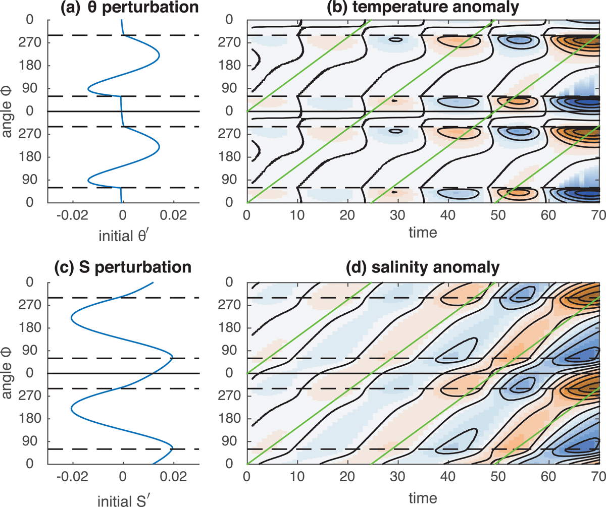
Figure 5.
Time evolution of an oscillatory instability. The initial temperature and salinity perturbations from the state C of Case 1 (no applied torque, see Table 1 and Fig. 3) are shown in panels (a) and (c), respectively. Initial perturbations correspond to the most unstable mode, scaled so that the velocity perturbation equals 0.01. Temperature and salinity anomalies as a function of time are shown in panels (b) and (d), respectively. Anomalies are defined as the difference with the distributions of steady state C. As the anomaly signal propagates around the loop, it amplifies exponentially. The phase of the anomaly as predicted by linear theory is shown in green.
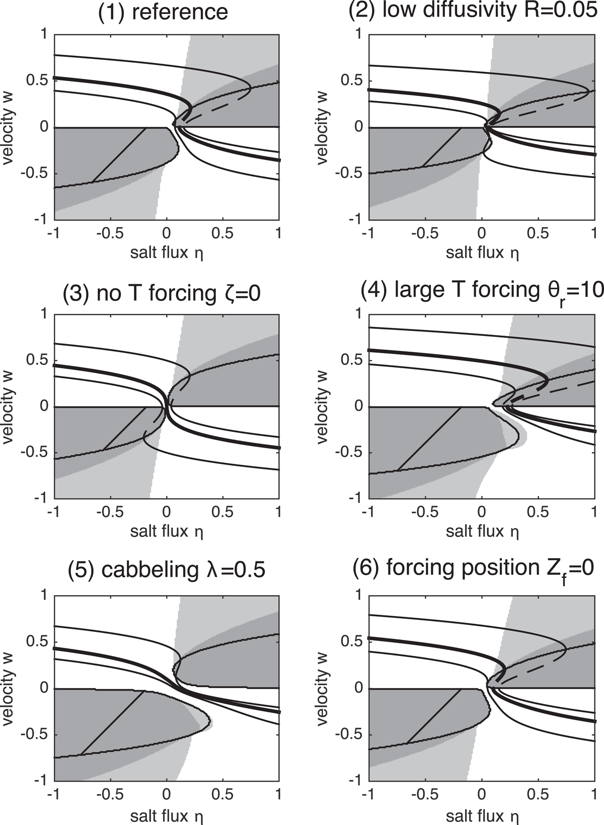
Figure 6.
Bifurcation diagrams for a variety of configurations (listed in Table 1). The bifurcation diagram indicates, based on the linear stability analysis, ranges of [white] stability, [light grey] oscillatory instability and [dark grey] torque instability. Regions of torque instability based on the simple instability criterion are hatched, showing that this criterion tends to underestimate the actual domain of torque instability. Each case differs from the reference case by only one modified parameter. The steady-state velocity for a zero applied torque follows the thick black contour. Thin contours associated with and are also superimposed, found above and below the zero contour, respectively.
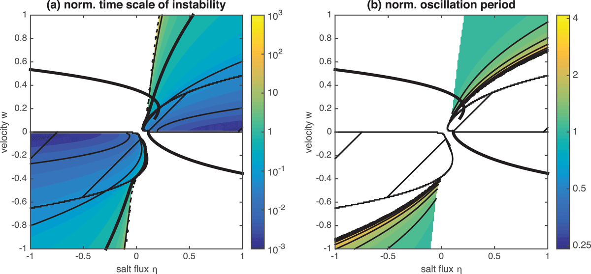
Figure 7.
(a) Ratio between the e-folding scale of instability and the revolution time (in logarithmic scale) for Case 1, showing that instabilities develop much faster in the domain of torque instability than for oscillatory instabilities. (b) Ratio between the oscillation period and the revolution time (in logarithmic scale) for Case 1, defined only for oscillatory states. The oscillation period is generally of same order of magnitude as the revolution timescale.
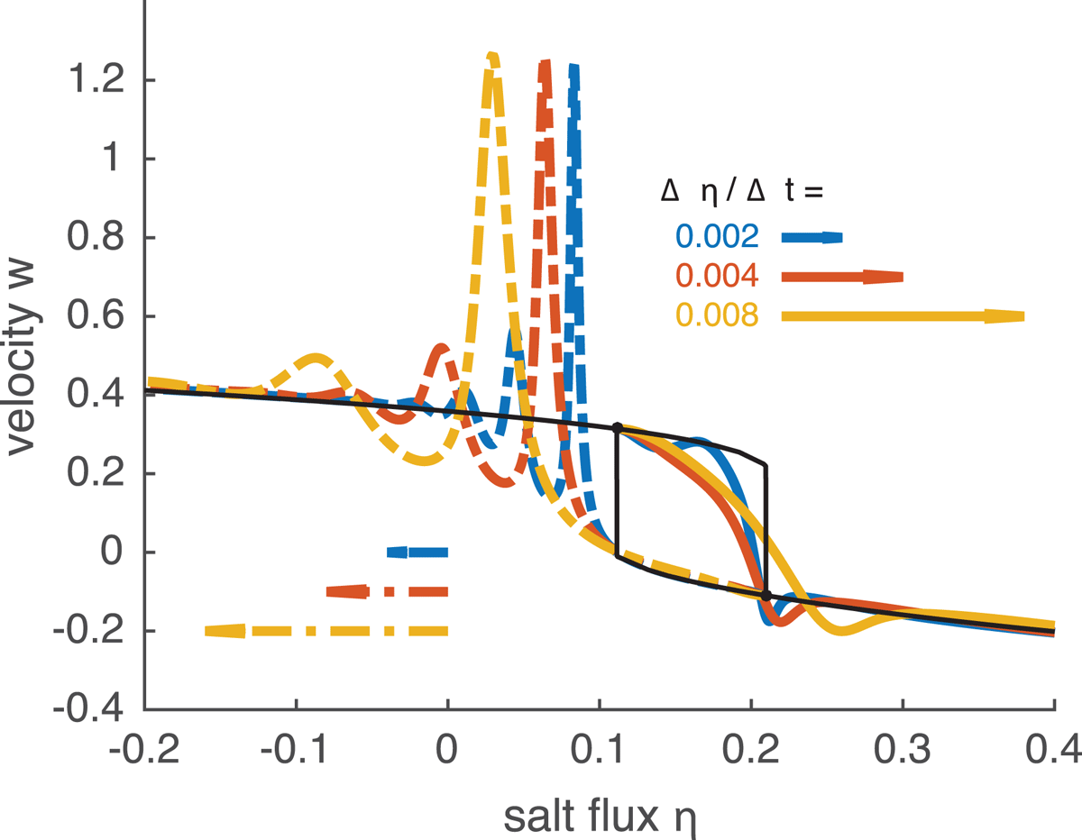
Figure 8.
Transitory response when the salt flux parameter is varied linearly at different time rates ( 0.002 in blue, 0.004 in red and 0.008 in yellow), starting from the fast mode and increasing the salt flux (solid lines), or starting from the slow mode and decreasing the salt flux (dashed lines). The theoretical fast and slow steady-state velocities are superimposed (black solid lines). When the salt forcing is increased starting from the fast mode, the velocity starts to decrease before it reaches the turning point due to the development of an oscillatory instability. By contrast, when the salt is decreased starting from the slow mode, the recovery begins only after the turning point has been passed.