
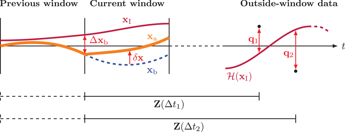
Figure 1.
The proposed method to incorporate lagged covariances for the case in which future data influence the current assimilation trajectory. The thin burgundy line indicates the analysis produced in the first assimilation run (), the dashed blue line indicates the background in the second assimilation run () and the thick orange line indicates the analysis in the second assimilation run (). The innovations between the future data and (the model state transformed into observation space) are denoted and are separated from the start of the current assimilation window by lags . The innovations, together with the matrices , are used to influence the increments () at the start of the current window. The difference between the first and second assimilation runs at this point () must be considered when determining . The dashed extensions to indicate the lags that were used for the assimilation in the previous window, for which the corresponding may be different.
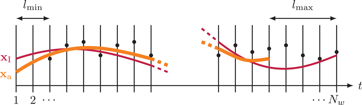
Figure 2.
The times spanned by the outside-window data and the assimilation trajectories in the simulation study. The first assimilation stage, which produces the trajectory (thin burgundy line), spans assimilation windows (indicated on the x-axis). The outside window data (black points) span times between and and are generated at the start of each window. The second assimilation stage spans times between 1 and and produces the trajectory (thick orange line). In each window the outside-window data between and in the future influence the trajectory.
Table 1.
Mean and standard deviation of the assimilation metric for different scenarios. The metric and scenarios are described in the text.
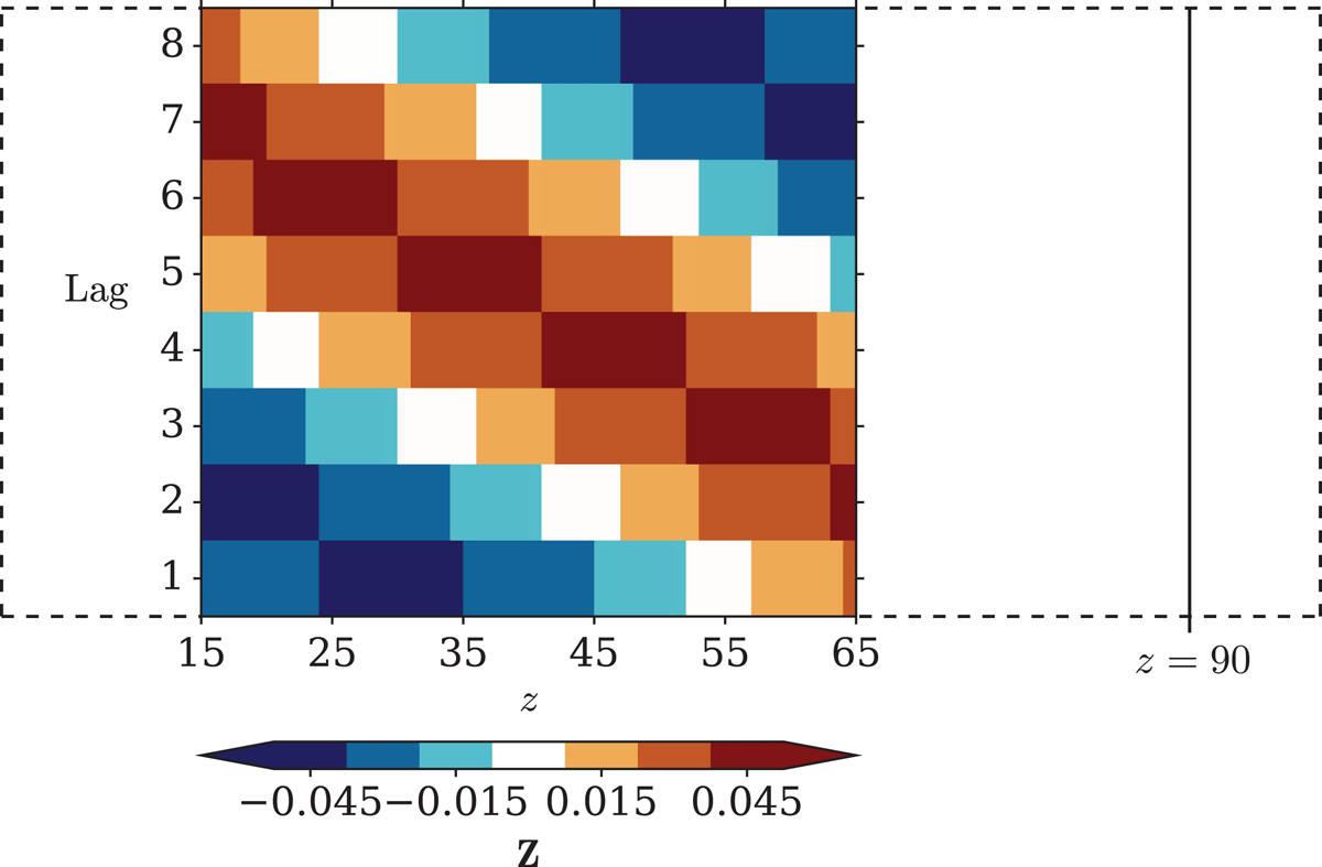
Figure 3.
Values of as a function of spatial coordinate (z) and lag (in multiples of 10 time units). Lags from 10–80 time units are considered and the z-values are restricted to the spatial domain of the increments influenced by the outside-window data. The dashed lines show the full spatial extent of the domain and the vertical line marks .
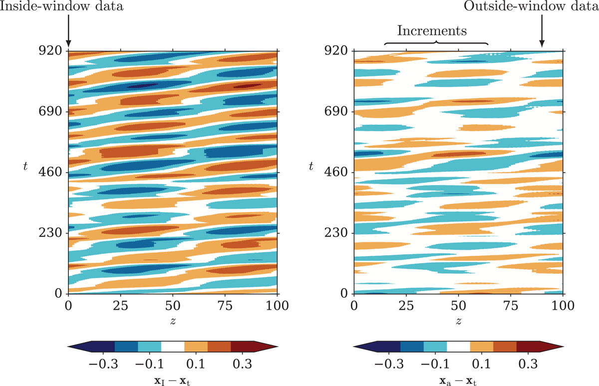
Figure 4.
The difference between (left) the initial assimilation and the truth (right) the second assimilation and the truth for one realisation of scenario B. The spatial location of the within-window data is indicated on the left-hand plot. On the right-hand plot the locations of the outside-window innovations, and the increments that they influence, are shown.
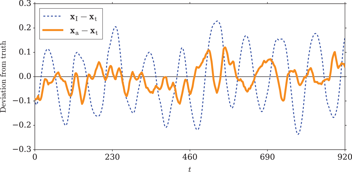
Figure 5.
Time evolution of deviations between the truth and the (dashed blue line) first (thick orange line) second assimilation trajectory at for one realisation of scenario B.
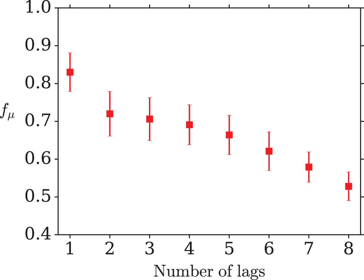
Figure 6.
The dependence of the metric on the number of lags used in the assimilation.
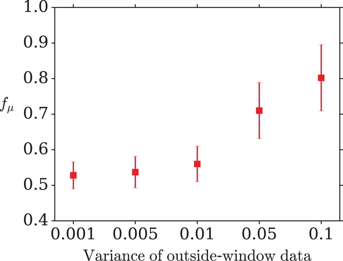
Figure 7.
The dependence of the metric on the error variance of the outside-window observations.

Figure 8.
The difference between (left) the initial assimilation and the truth (right) the second assimilation and the truth for one realisation of scenario D. On the right-hand plot the locations of the outside-window innovations, and the increments that they influence, are shown. The quantities on the left-hand plot extend to approximately .
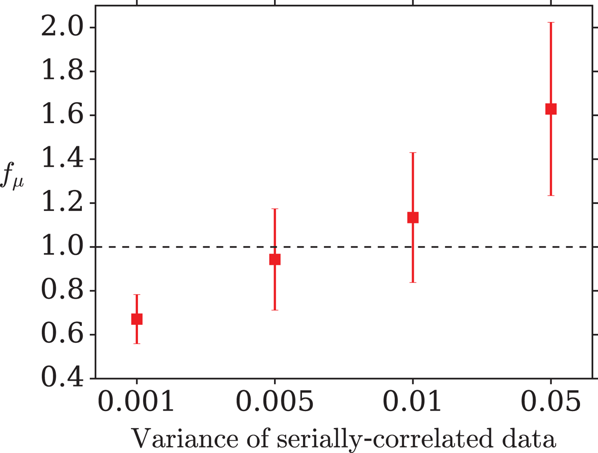
Figure 9.
The dependence of the metric on the error variance of the serially correlated outside-window observations.
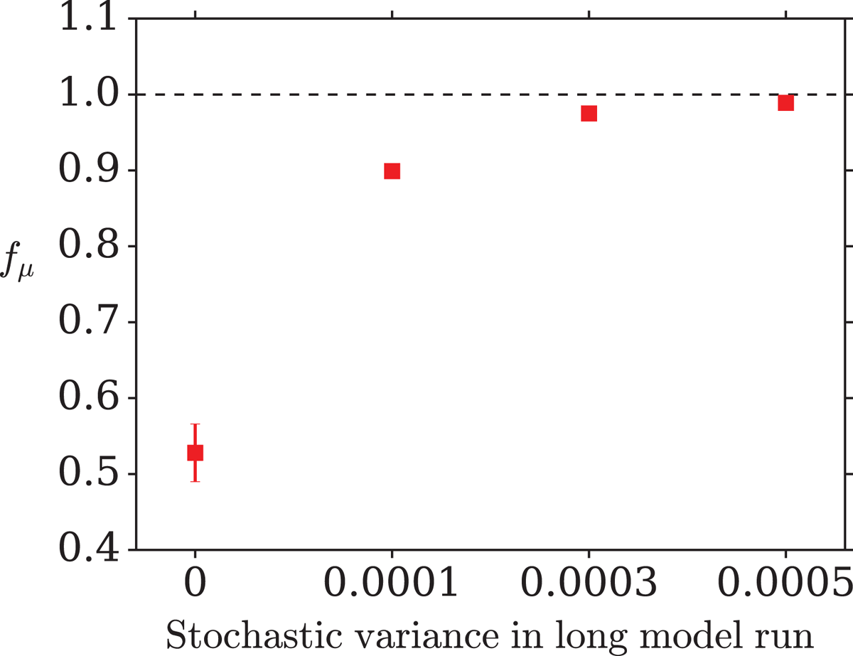
Figure 10.
The dependence of the metric on the stochastic variance of the long model run used to determine the matrices.
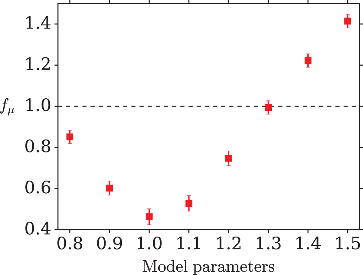
Figure 11.
The dependence of the metric on the parameters of the long model run used to determine the matrices. In each case, both the amplitude and speed of the model are set to the same value.
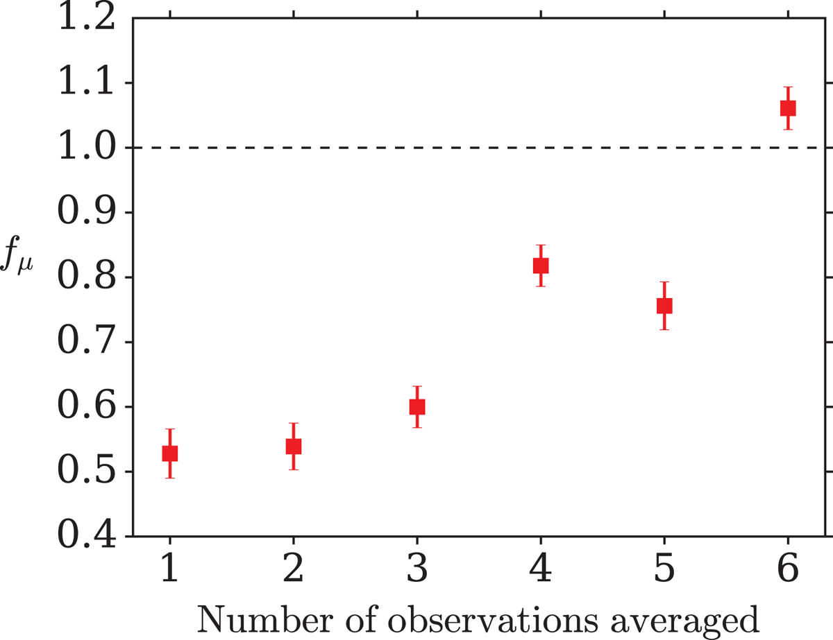
Figure 12.
The dependence of the metric on the number of consecutive outside-window observations which are averaged together.
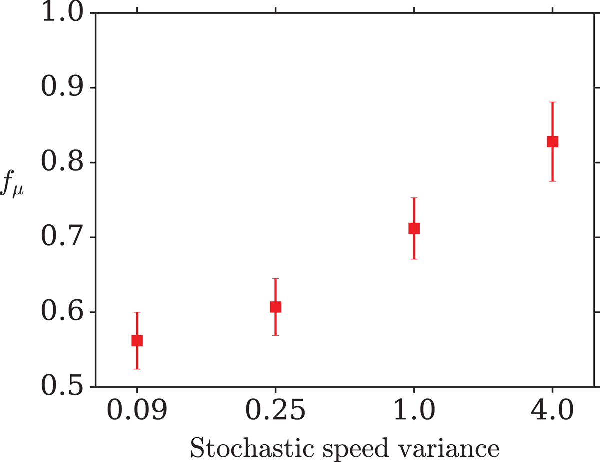
Figure 13.
The dependence of the metric on the stochastic speed variance.
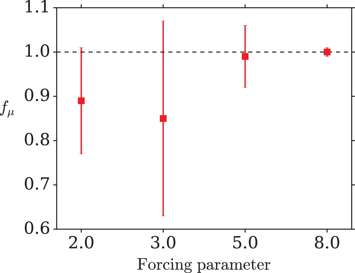
Figure 14.
The dependence of the metric on the ‘Lorenz 96’ model forcing parameter.