
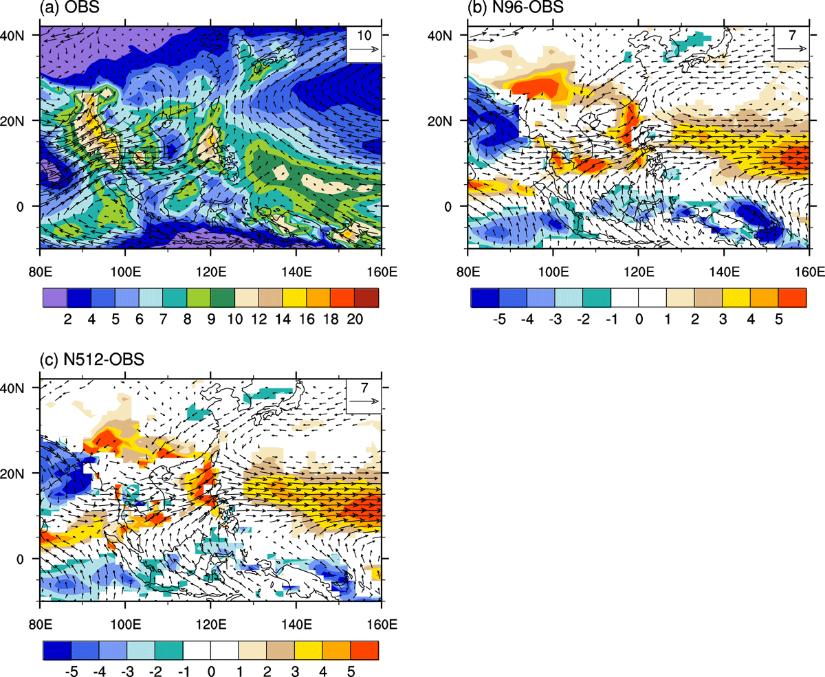
Fig. 1.
May–September mean rainfall (shaded, units: mm day−1) and 850 hPa wind vectors from the (a) Observation, (b) the difference between N96 and observations and (c) the difference between N512 and observations. Only the regions where the difference of precipitation and wind vectors are statistically significant at 5% level (Student’s t test) are plotted in (b) and (c).
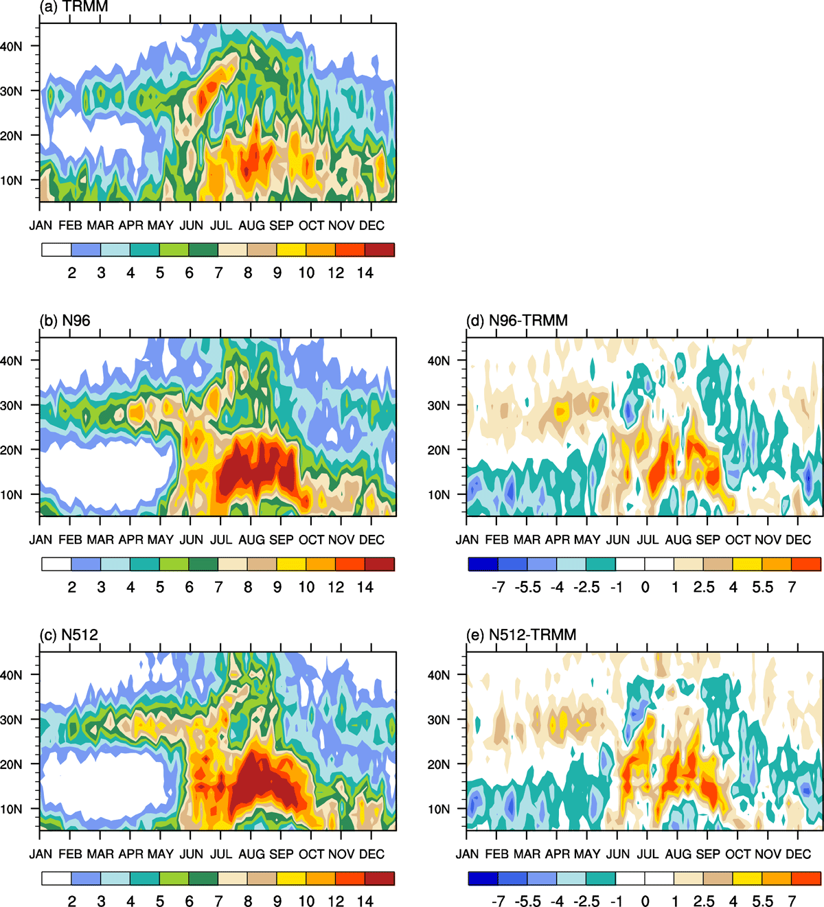
Fig. 2.
Annual cycle climatology for rainfall rate (units: mm day−1) averaged between 122 and 135°E from (a) TRMM 3B42, (b) N96, (c) N512, (d) the difference between N96 and observations and (e) the difference between N512 and observations.
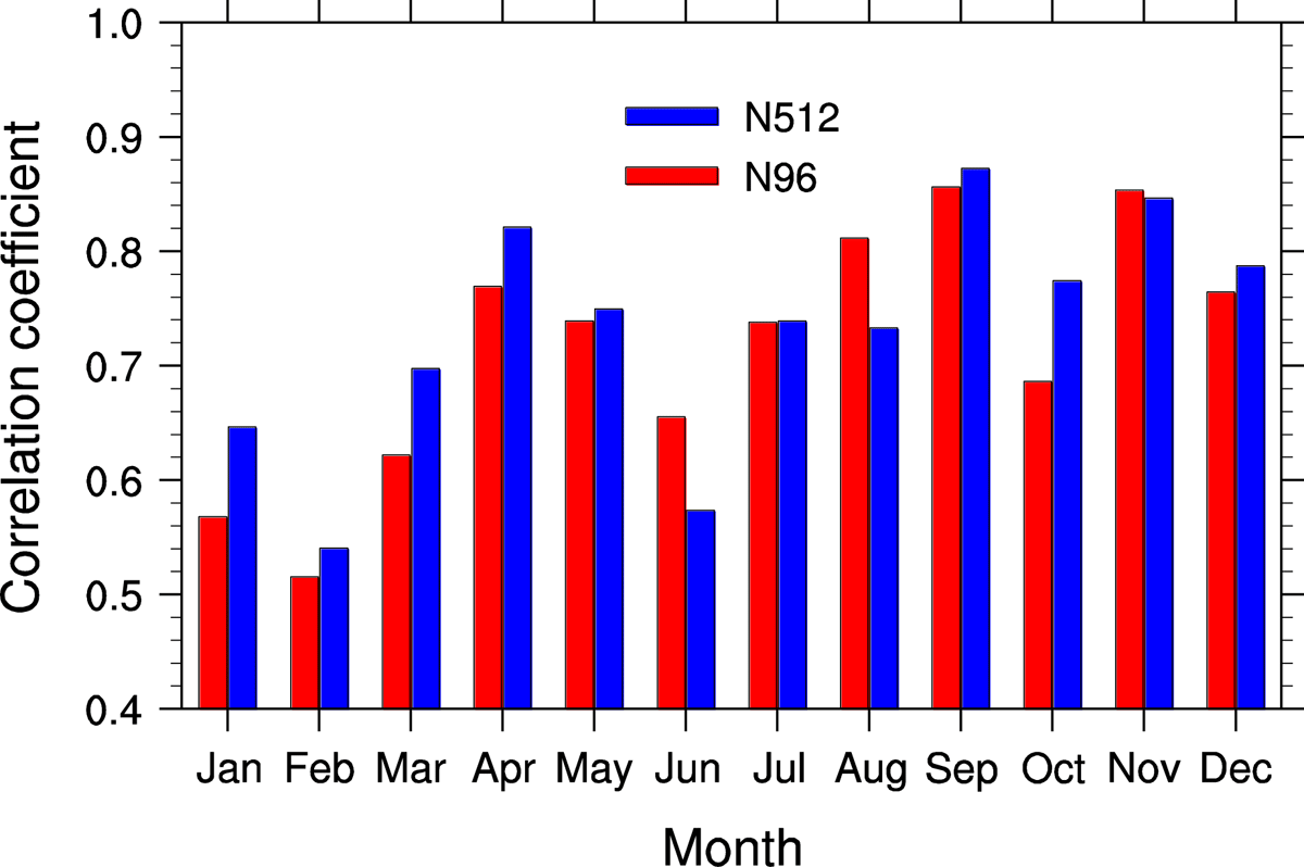
Fig. 3.
Spatial pattern correlation coefficient of month mean precipitation between the observation and simulations over the EAWNP region.
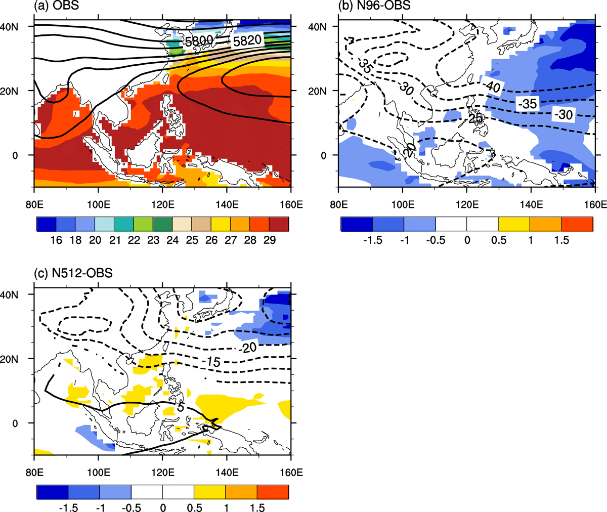
Fig. 4.
May–September mean SST (shaded, units: °C) and 500 hPa geopotential height (contour, units: gpm) from the (a) Observation, (b) the difference between N96 and observations and (c) the difference between N512 and observations. Only the regions where the difference of SST and 500 hPa geopotential height are statistically significant at 5% level (Student’s t test) are plotted in (b) and (c).
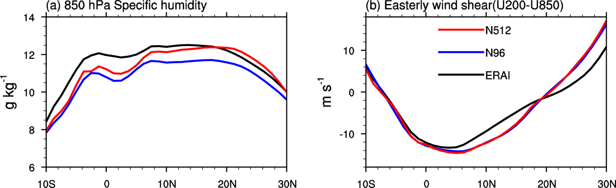
Fig. 5.
Meridional distribution of May–September mean (a) 850 hPa specific humidity and (b) easterly wind shear between 200 and 850 hP averaged between 122 and 135°E.
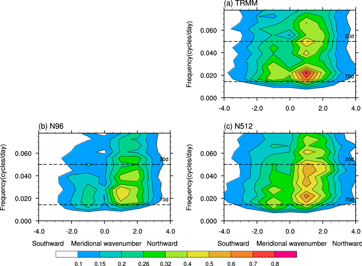
Fig. 6.
Meridional wavenumber-frequency spectra during boreal summer over 15°S–30°N using precipitation (units: mm−2 day−2) averaged between 122 and 135°E from (a) TRMM 3B42, (b) N96 and (c) N512.
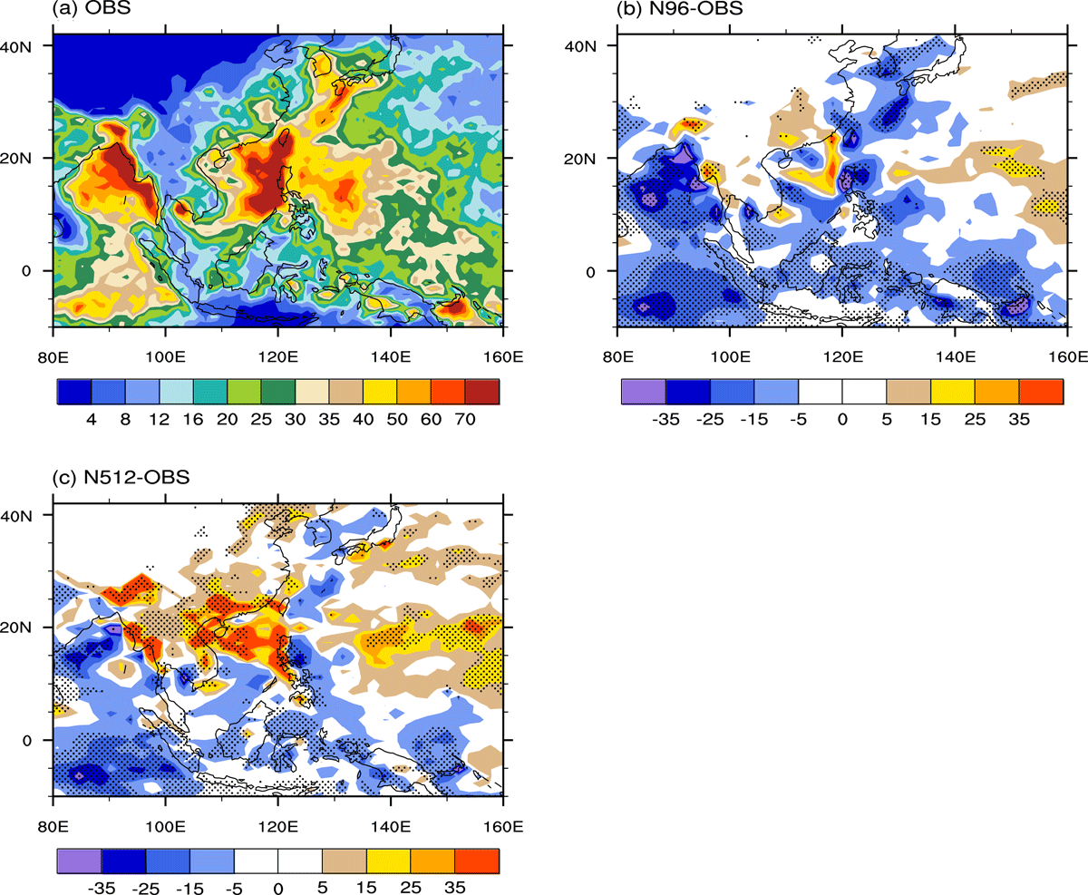
Fig. 7.
20–70 day filtered precipitation variance (units: mm2 day−2) during boreal summer (May–September) for the (a) Observation, (b) the difference between N96 and observations and (c) the difference between N512 and observations. The stippling in (b) and (c) denotes where the difference of the intra-seasonal precipitation variance is statistically significant at 10% level according to a F-test.
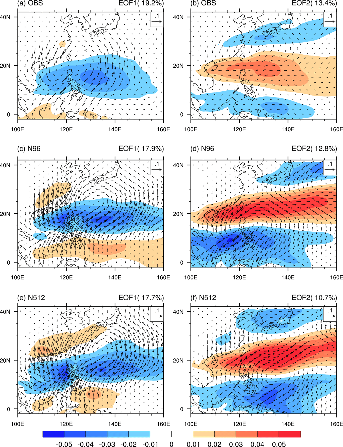
Fig. 8.
First two leading combined EOF modes of daily OLR (shading) and U850 anomalies from the (a) Observations, (b) N96 and (c) N512. To display the full horizontal wind vector, the associated 850-hPa meridional wind was obtained by regressing 850-hPa meridional wind anomaly against each PC.
Table 1.
Number of days for each phase of the monsoon ISO.
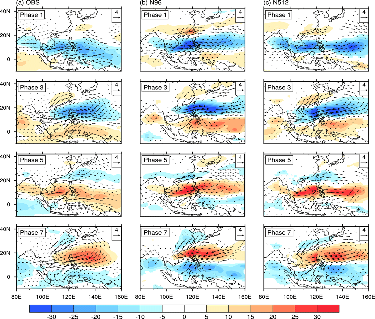
Fig. 9.
Composites of OLR (shaded, units: W m−2) and 850 hPa wind anomalies (vectors, units: m s−1) for phase 1, 3, 5 and 7 from (a) NOAA and ERAI reanalysis (left), (b) N96 (middle) and (c) N512 (right) simulations. Only the values of wind and OLR that significantly exceed the 95% confidence level are shown.
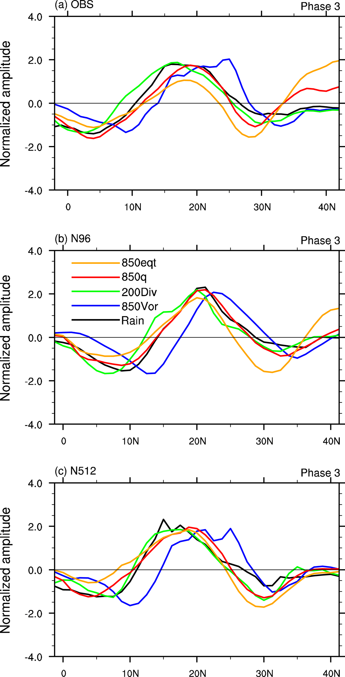
Fig. 10.
Meridional distribution of composite rainfall, 200 hPa divergence, 850 hPa equivalent potential temperature, specific humidity and vorticity at phase 3 for (a) Observation, (b) N96 and (c) N512. All variables are averaged over the 122–135°E and normalised by their respective standard deviations.
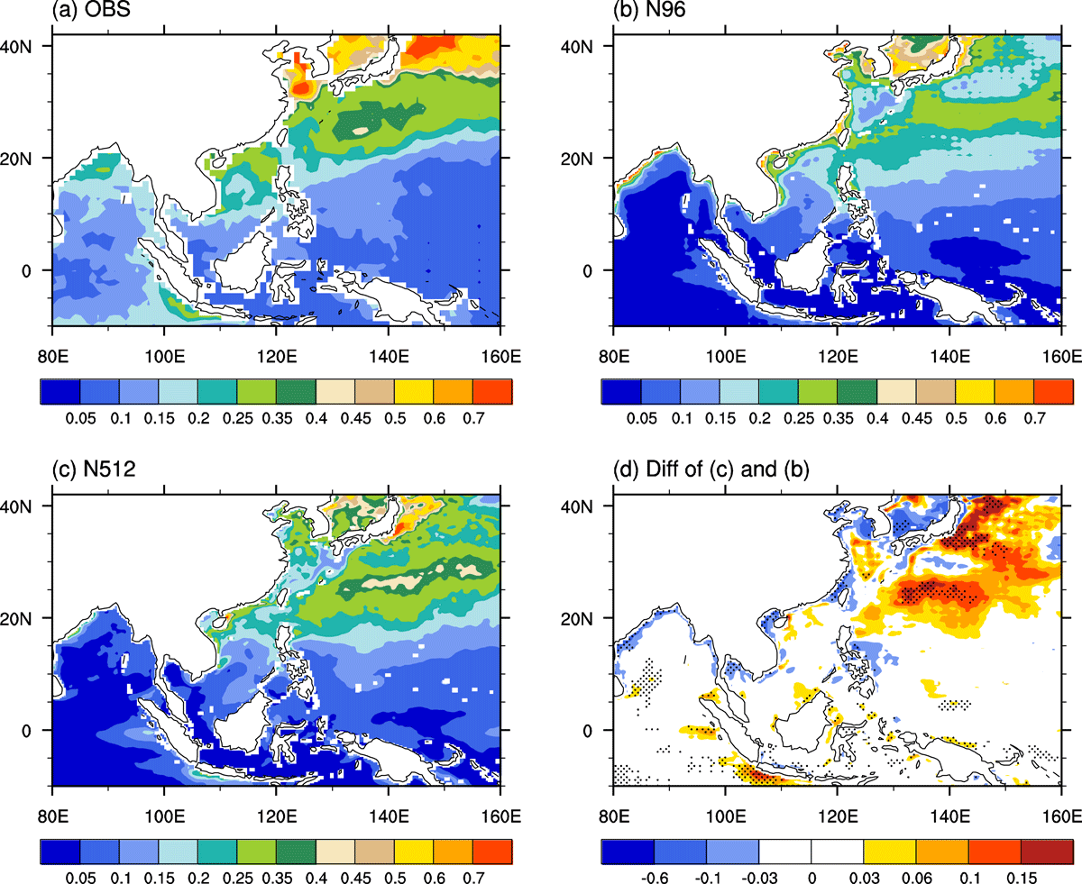
Fig. 11.
Composites of 20–70 day filtered 500 hPa (shading, units: gpm) and 200 hPa (contour with an interval of 4 gpm) geopotential height over the EAWNP region at phase 1 (left) and 5 (right) for (a) and (b) ERAI reanalysis, (b) and (c) N96, and (e) and (f) N512.
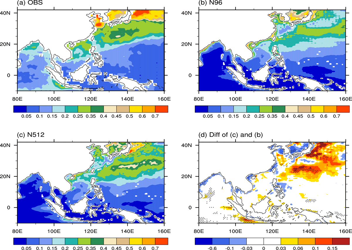
Fig. 12.
20–70 day filtered SST variance (units: °C) during boreal summer (May–September) for the (a) OBS, (b) N96, (c) N512 and (d) the difference between N512 and N96. The stippling in (d) denotes where the difference of the intra-seasonal SST variance is statistically significant at the 10% level according to a F-test.
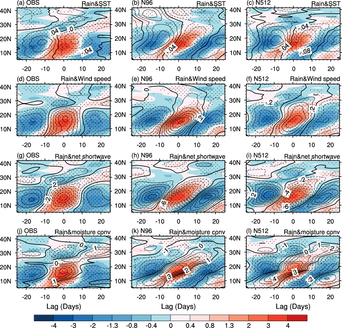
Fig. 13.
Lag regression of the 20–70 day filtered precipitation (shaded, units: mm day−1), SST (contours with an interval of 0.04 °C), 850 hPa wind speed (contours with an interval of 0.2 m s−1), surface net downward shortwave flux (contours with an interval of 2 W m−2) and 1000-hPa moisture convergence (contours with an interval of 1 × 10⁻⁹ kg s−1 kg−1) along 122–135°E upon the filtered precipitation averaged over the South China Sea and Philippine Sea (10–20°N, 110–130°E) for (a, d, g, j) observation, (b, e, h, k) N96 and (c, f, i, l) N512. The stippling indicates the regions where both regression coefficients are statistically significant at the 5% significance level.