
Table 1.
Overview of models used in this study. H/L refers to the magnitude of change in the global average temperature, precipitation and wind speed during the twenty-first century. In the case of temperature and precipitation the definition of H and L is directly related to the ECS, with a breakpoint at 3.5.
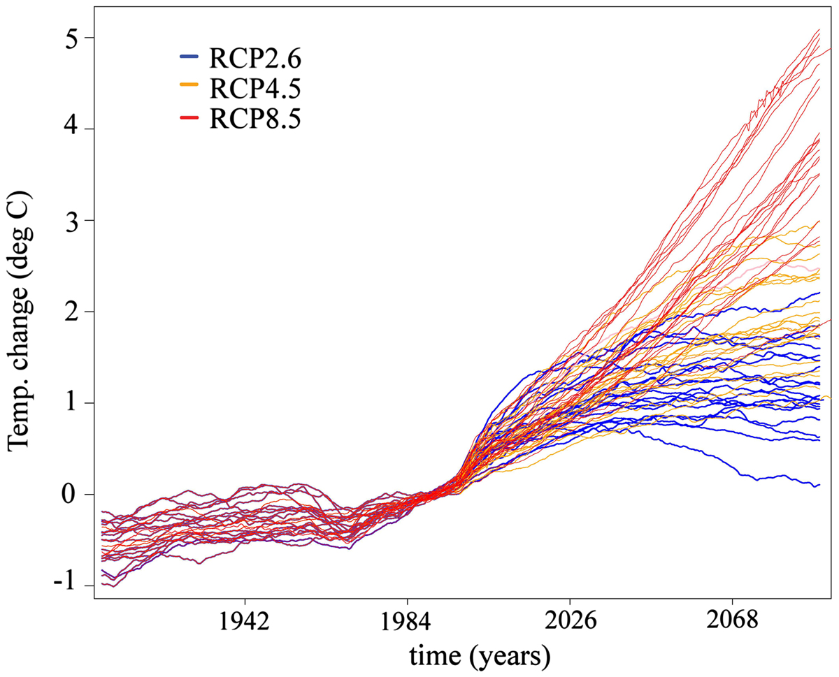
Fig. 1.
Global surface temperature anomaly relative to the 1971–1999 period. One line for each model simulation in Table 1, using a 10-year moving average filter. Each scenario is shown in a different colour: RCP2.6 in blue, RCP4.5 in orange and RCP8.5 in red.
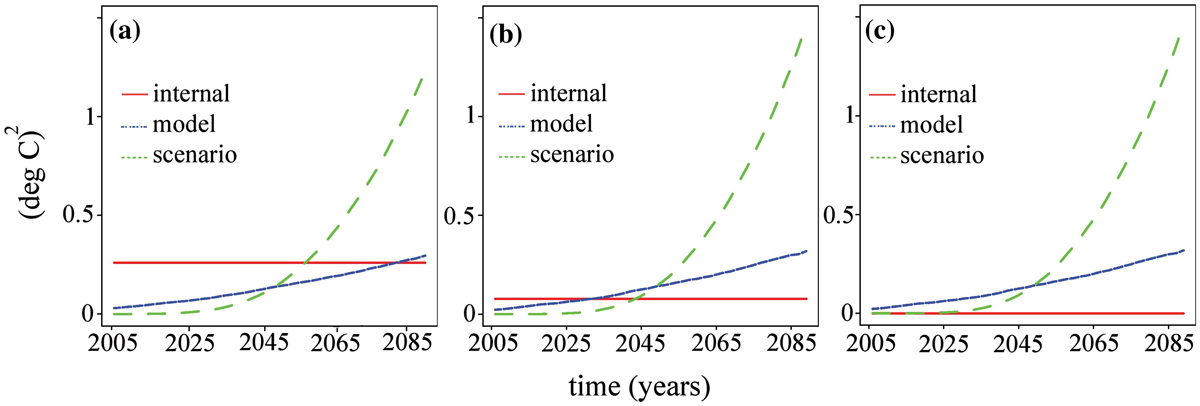
Fig. 2.
Climate projections uncertainty in temperature, using all models and all scenarios in Table 1. (a) Using x in Equation (3), i.e. a 1-year average; (b) as in (a), but using a two-year average x 2; (c) as in (a) but using x 10.
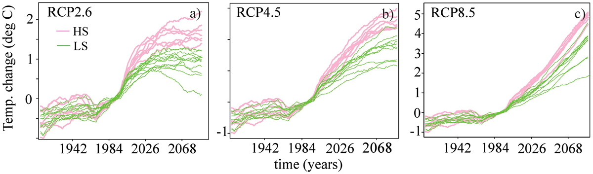
Fig. 3.
Global average surface temperature anomaly [°C] relative to the 1971–1999 period. Models with high ECS (HS; see Table 1, column 5) are coloured pink, low-sensitivity models (LS) coloured green. (a) Scenario RCP2.6; (b) RCP4.5; (c) RCP8.5.
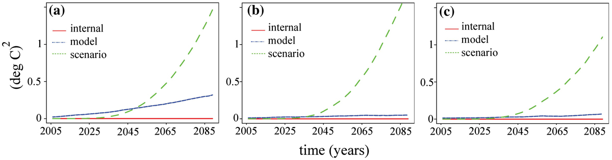
Fig. 4.
Climate projection uncertainty [(°C)2] for global mean air surface temperature: green (stippled) is scenario uncertainty, blue (dotted) is model uncertainty and red (solid) is internal uncertainty, following the method of (Hawkins and Sutton, 2009). The model runs used are listed in Table 1. The scenarios used are RCP 8.5, 4.5 and 2.6 (Moss et al., 2010). (a) Using all models in Table 1 (identical to Fig. 2c); (b) using only models with high ECS (see Table 1, models listed as H in Column 5; (c) using only models with low ECS (see Table 1, models listed as L in Column 5).
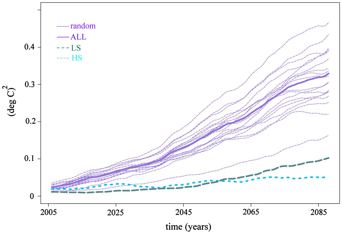
Fig. 5.
Model uncertainty for global average temperature change, calculated for various sets of model simulations from Table 1. In solid purple: using ALL models; in stippled green and dotted blue: the low-ECS (LS) and high-ECS (HS) model subsets (see column 5 of Table 1); in dash-dot purple: 20 randomly selected subsets of models from Table 1.
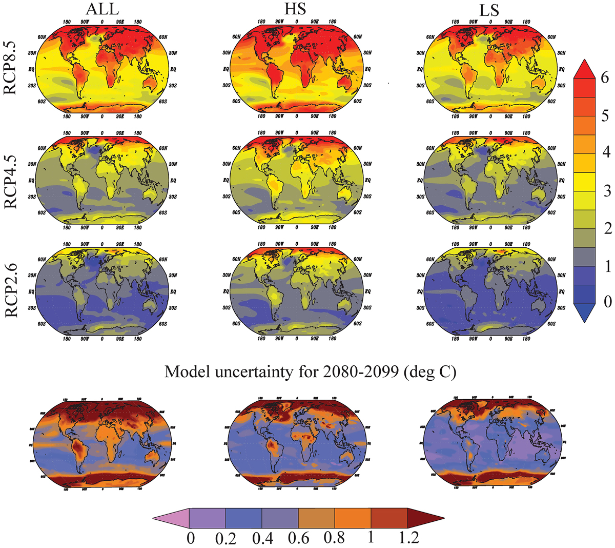
Fig. 6.
Multi-model ensemble mean projections of surface temperature anomalies for the 2080–2099 period relative to the 1971–1999 period [°C] and the square root of associated model uncertainties ([°C]; bottom row). Upper three rows: scenarios RCP 8.5, 4.5 and 2.6, respectively. Left column: using all models in Table 1; Middle column: using only high-sensitivity temperature projection models (see Table 1, models listed as H in Column 5; Right column: using low-sensitivity temperature projections models (see Table 1, models listed as L in Column 5).
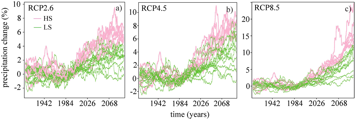
Fig. 7.
Global average precipitation anomaly [%] relative to the 1971–1999 period. High-ECS models (Table 1, Column 7) coloured pink, low-ECS models are coloured green. Only for one model, MRI-CGCM3, do we not use the ECS definition of sensitivity in precipitation; see note in Table 1. (a) Scenario RCP2.6; (b) RCP4.5; (c) RCP8.5.
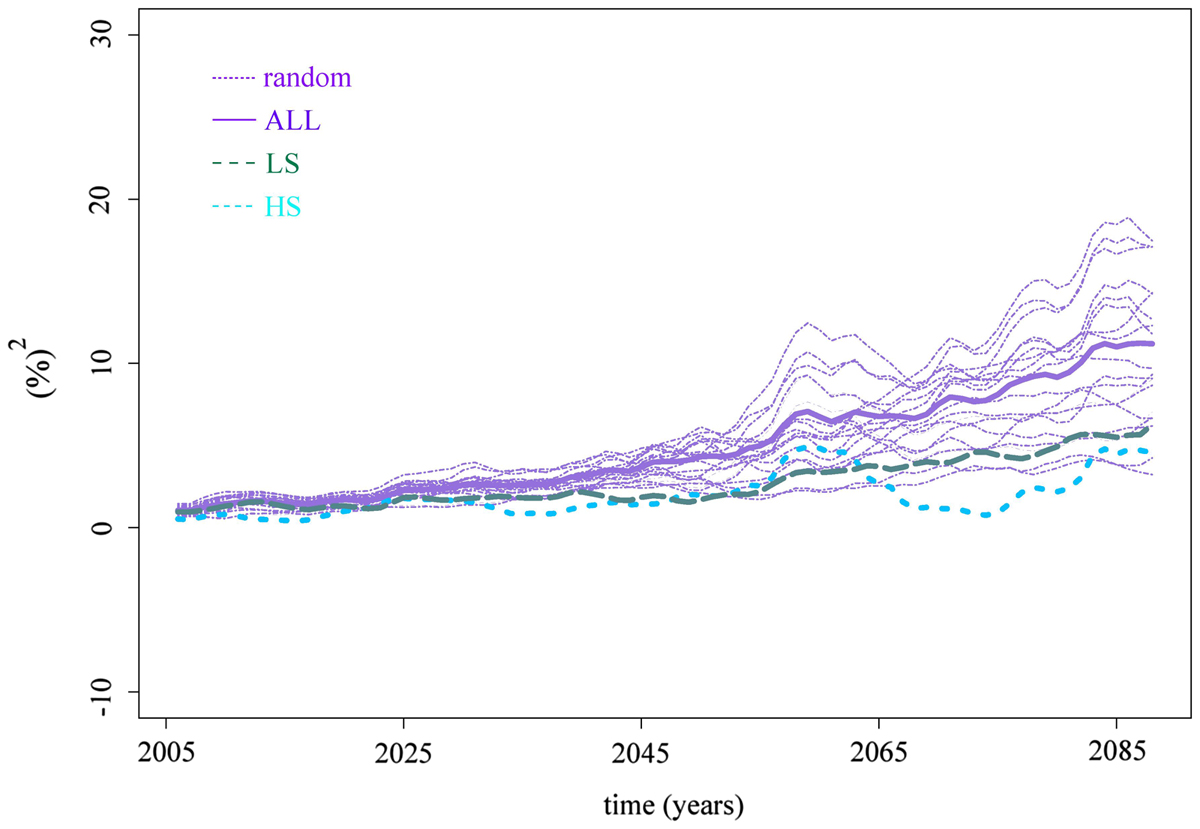
Fig. 8.
Model uncertainty for global average precipitation change, calculated for various sets of model simulations from Table 1. In solid purple: using ALL models; in stippled green and dotted blue: the LS and HS model sets (see column 7 of Table 1); in dash-dot purple: 20 randomly selected subsets of models from Table 1, with similar size as the HS and LS model sets.
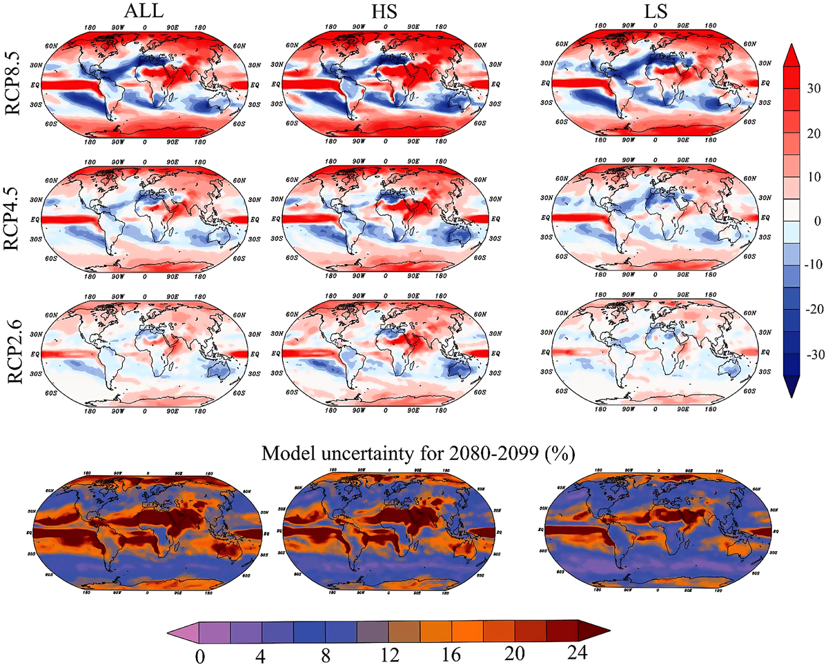
Fig. 9.
Same as Fig. 6 but for percentage precipitation change [%].
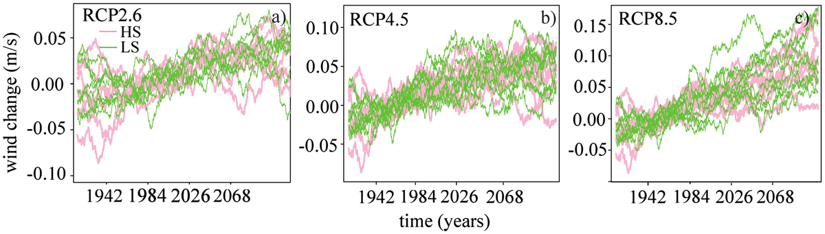
Fig. 10.
Global average wind speed anomaly [m/s] relative to the 1971–1999 period. High-ECS models (Table 1, Column 5, though note that we do not have the wind fields for all models – see Table 1, column 8) coloured pink, low-ECS models coloured green. (a) Scenario RCP2.6; (b) RCP4.5; (c) RCP8.5.
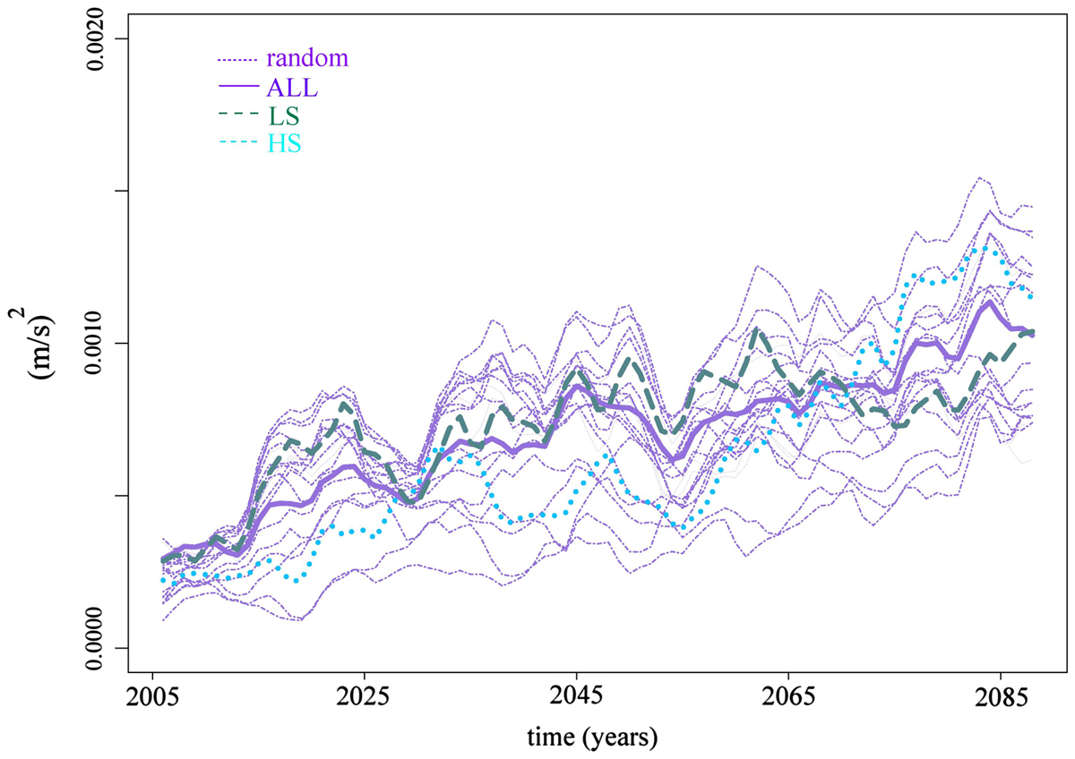
Fig. 11.
Model uncertainty for global average wind speed change, calculated for random sets of model simulations from Table 1. In solid purple: the average of all the models; in stippled green and dotted blue: the LS and HS model sets (as in Fig. 10); in dash-dot purple: 20 randomly selected subsets of models from Table 1, with similar size as the HS and LS model sets.
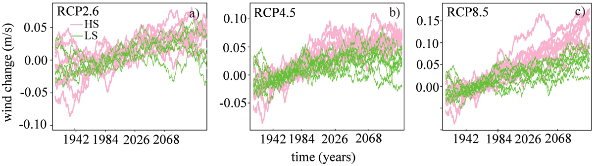
Fig. 12.
Global average wind speed anomaly [m/s] relative to the 1971–1999 period. High-sensitivity models (determined by each model’s global average wind speed change in the twenty-first century; see Table 1, Column 9) coloured pink, low-sensitivity models colored green. (a) Scenario RCP2.6; (b) RCP4.5; (c) RCP8.5.
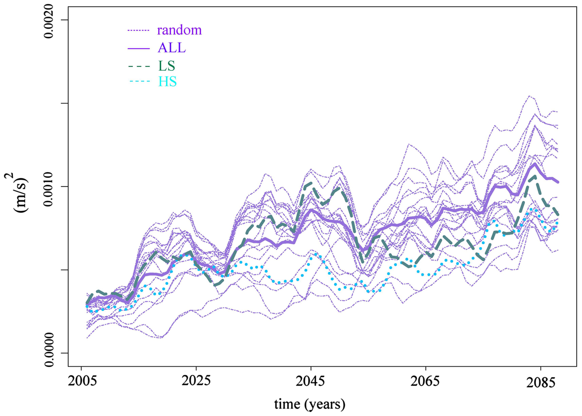
Fig. 13.
Model uncertainty for global average wind speed change, calculated for various sets of model simulations from Table 1. In solid purple: ALL models; in stippled green and dotted blue: The L and H models sets based on wind-speed change (see Fig. 12 and column 9 of Table 1); in dash-dot purple: 20 randomly selected subsets of models from Table 1, with similar size as the H and L model sets.
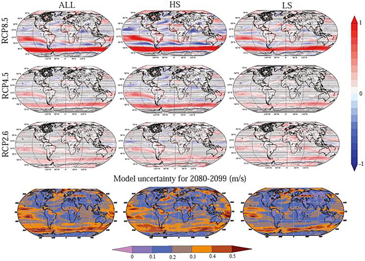
Fig. 14.
Same as Fig. 6 but for wind speed change [m/s]. Since the model uncertainties are of the same order of magnitude as the projected change in the case of wind speed, we have overlaid a mask indicating change that is not significantly larger than the uncertainty. Specifically, it is the result of a two-sided rank sum test with p-values showing the null hypothesis is not valid; i.e. the hatching shows areas where there is no significant change for the 2071–2099 period relative to the baseline period (1971–1999) at a 95% level.