
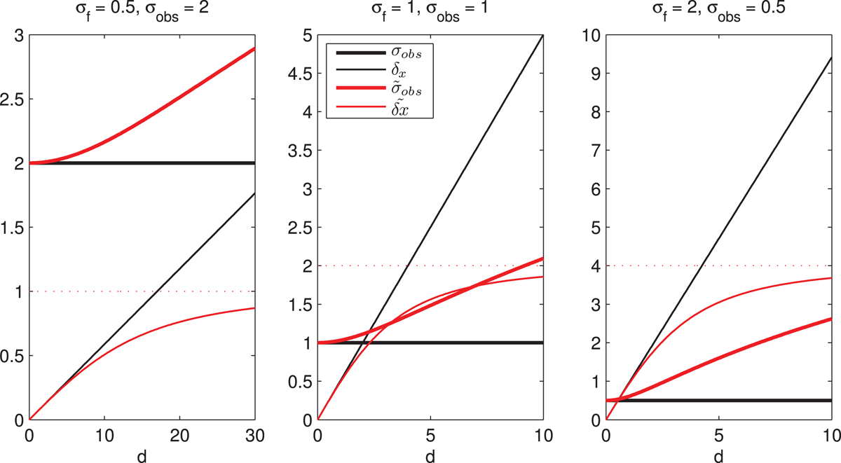
Figure 1.
Behaviour of the solution (12) for (thick red line) and the associated increment (thin red line) vs. innovation d; calculated for three combinations of observation error variance and state error variance in the case . The black lines show non-modified variables and , and the dotted red lines indicate the maximal achievable increment of .
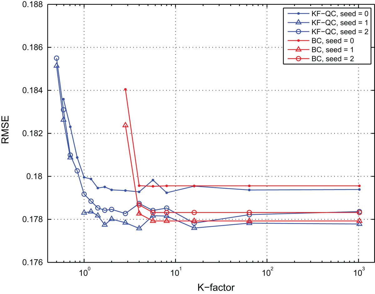
Figure 2.
Mean analysis RMSE of a nearly optimal system with KF-QC and BC for three different initial conditions (seeds).
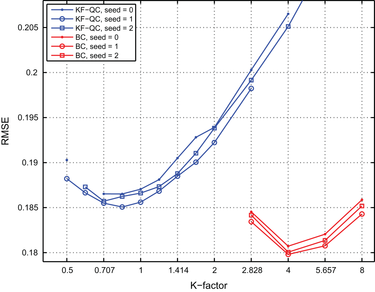
Figure 3.
Performance of a system with non-Gaussian dense observations using KF-QC and BC for three different initial conditions (seeds).
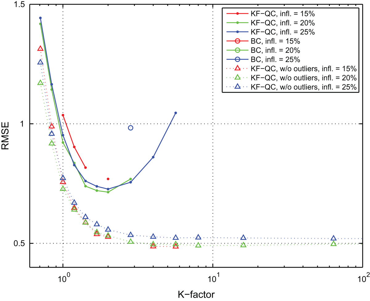
Figure 4.
Performance of a system with non-Gaussian sparse observations using KF-QC.
Table 1.
MAD of the forecast innovations for runs with different K-factors, averaged over all cycles.
Table 2.
Mean dissipated TKE over 3-day cycle, calculated as mean increment minus trend.
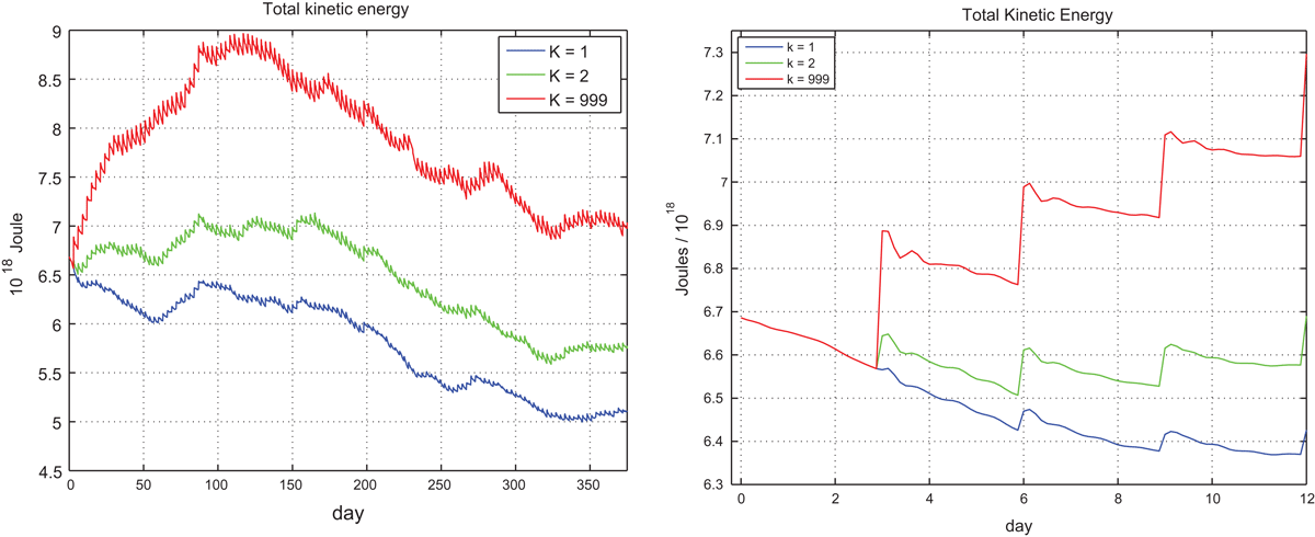
Figure 5.
Total kinetic energy for a realistic DA system with different K-factor values.
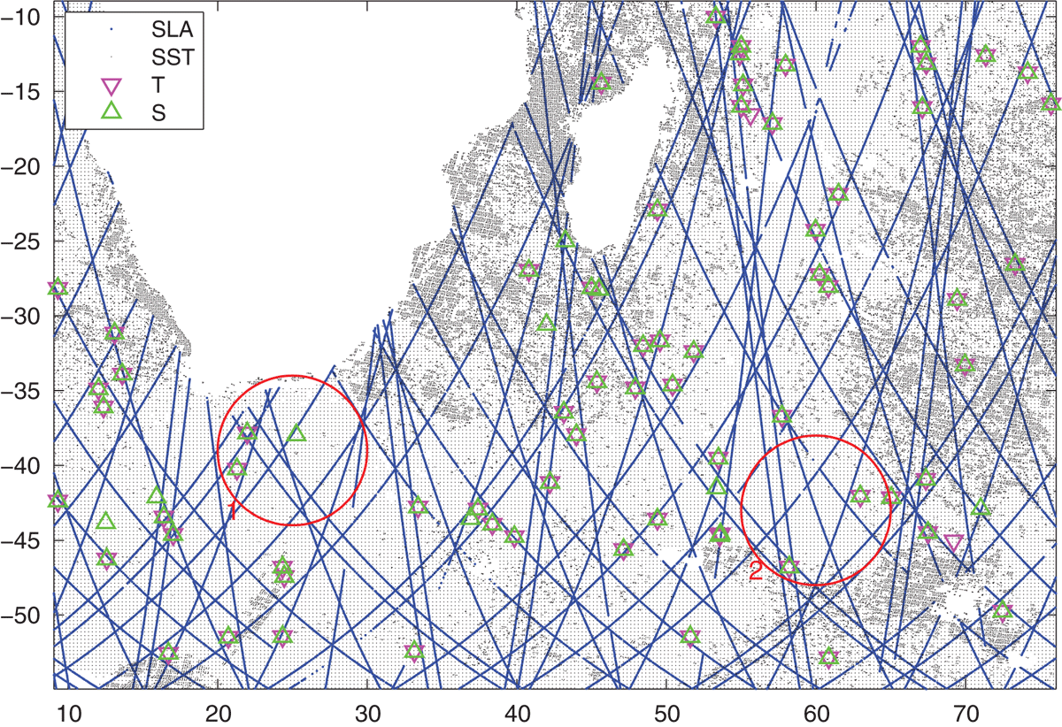
Figure 6.
Observations assimilated in analyses in Fig. 11, on 1 July 2011. The red circles correspond to the regions shown in Fig. 11.
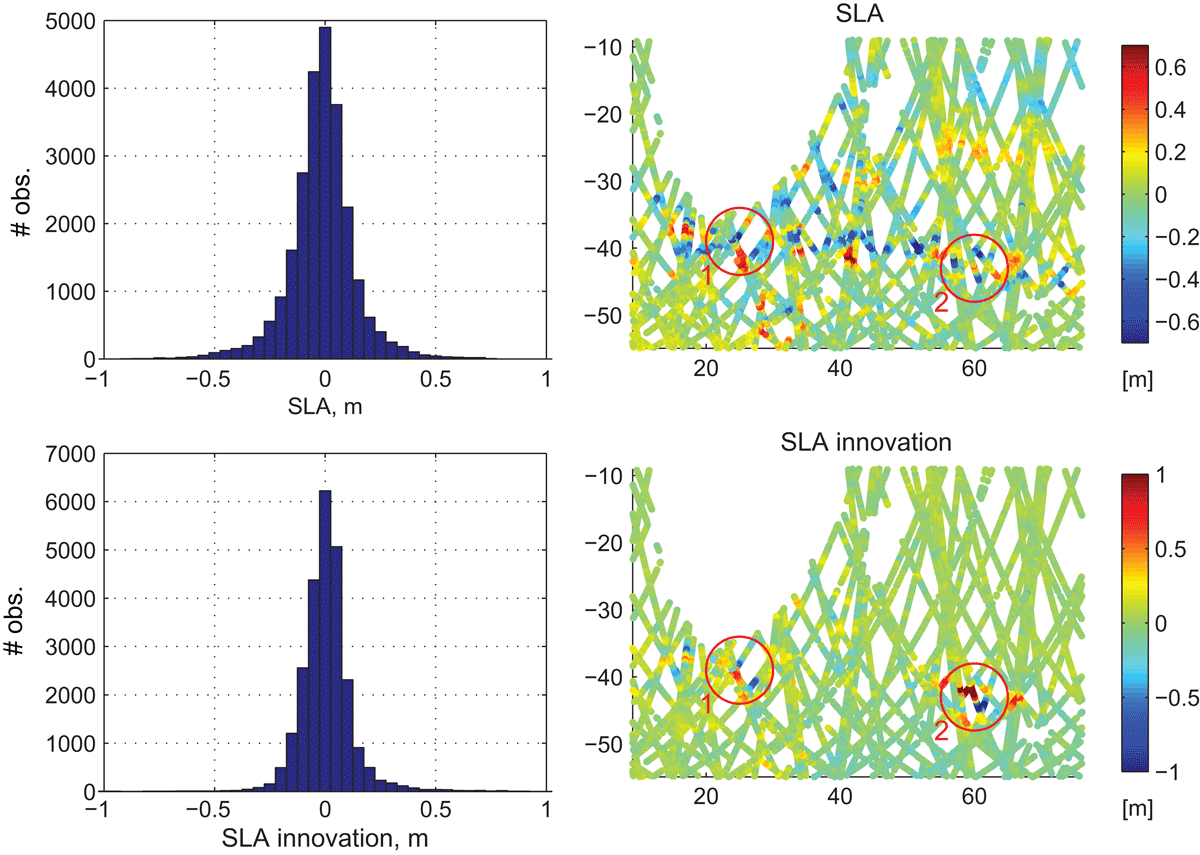
Figure 7.
SLA observations in Fig. 6.
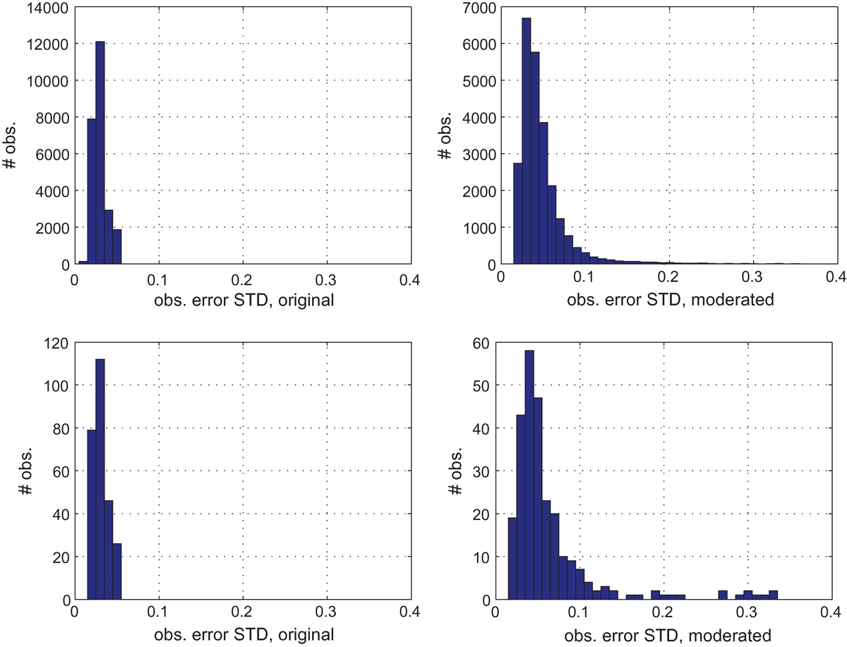
Figure 8.
Observation error for SLA observations in Fig. 6 before and after applying the KF-QC with , for all SLA observations (upper row) and for observations with innovation magnitude exceeding 0.5 m (lower row).
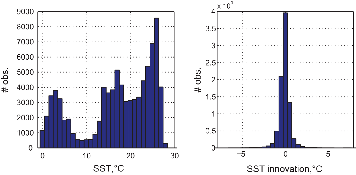
Figure 9.
Histograms of SST observations in Fig. 6.
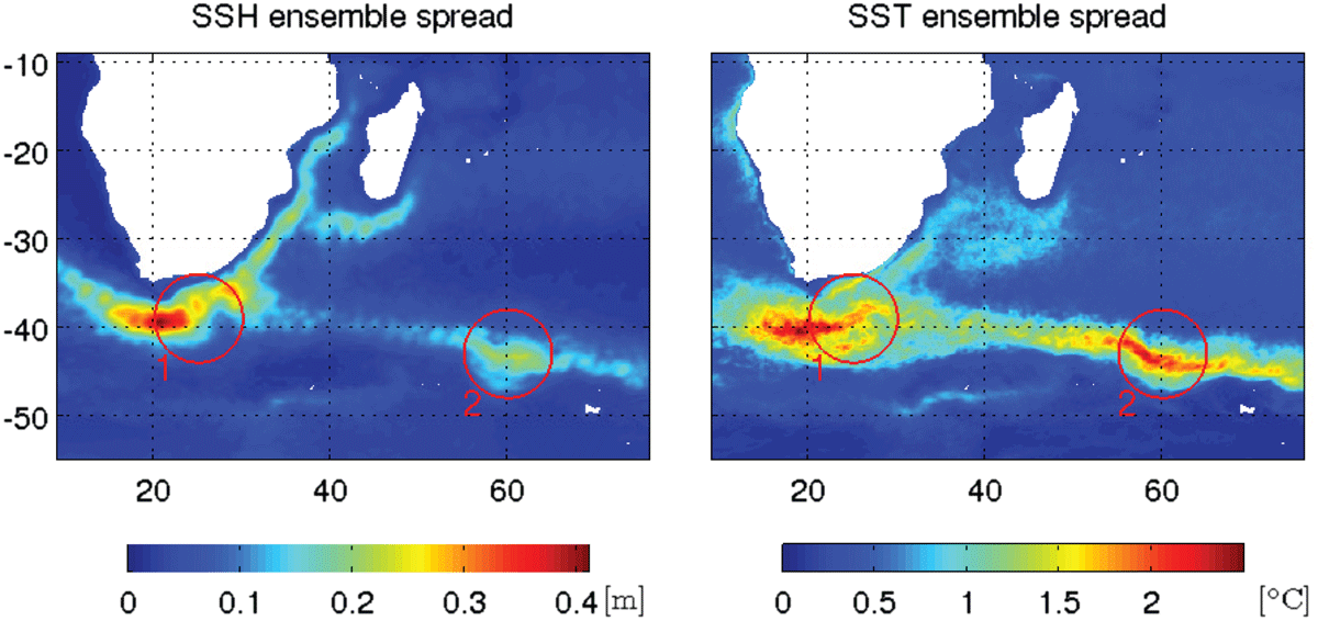
Figure 10.
Sea surface height and SST ensemble spread in the ocean DA system.
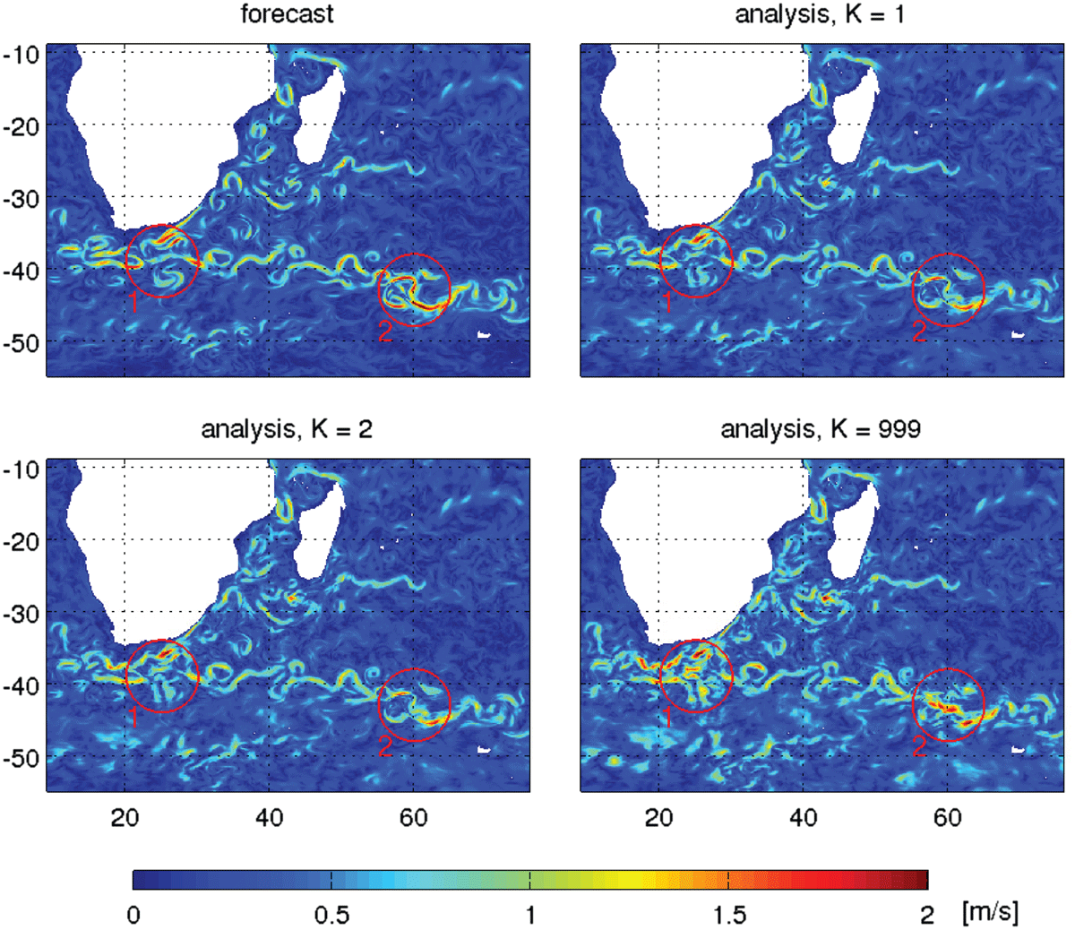
Figure 11.
Surface velocity magnitude in a realistic ocean DA system: the forecast, and analyses obtained with different K-factors.