
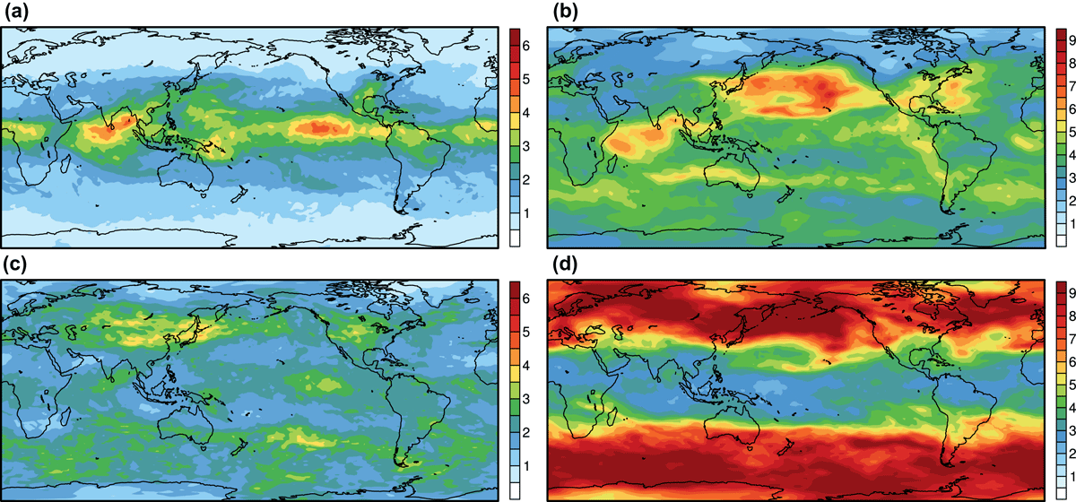
Figure 1.
Growth of the global forecast uncertainties. Ensemble spread in May 2015 ECMWF ENS for zonal wind at (a–b) model level 45 (around 150 hPa) and (c–d) model level 55 close to 300 hPa in (a,c) 24-h forecasts and (b,d) 120-h forecasts. Colourbar is in m/s.
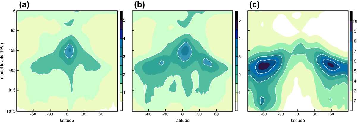
Figure 2.
As in Fig. 1 but for the zonally averaged zonal wind spread in (a) 12-h forecast, (b) 24-h forecast and (c) 120-h forecast.
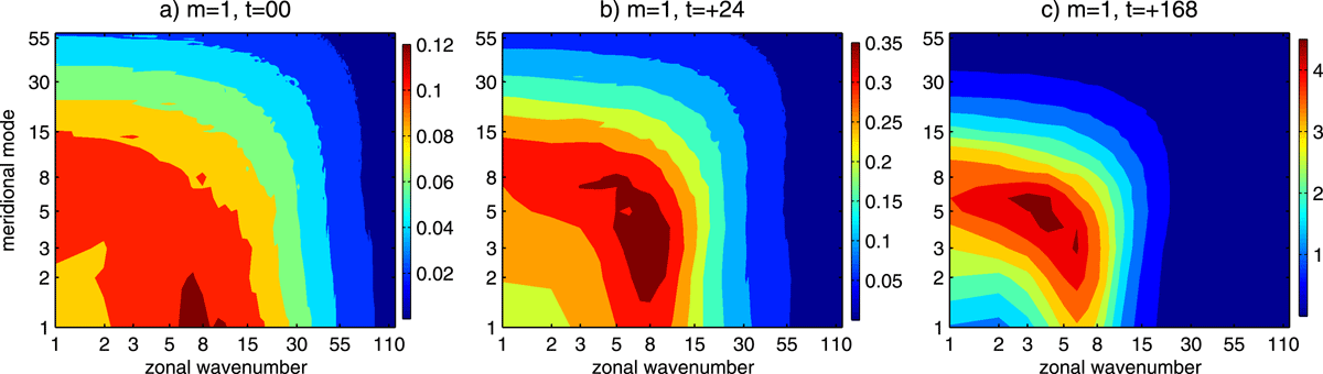
Figure 3.
Ensemble spread as a function of the zonal wavenumber and meridional mode for the balanced vertical mode at (a) initial time, (b) 24-h forecast, and (c) 7-day forecast. Colourbar is in meters per second.
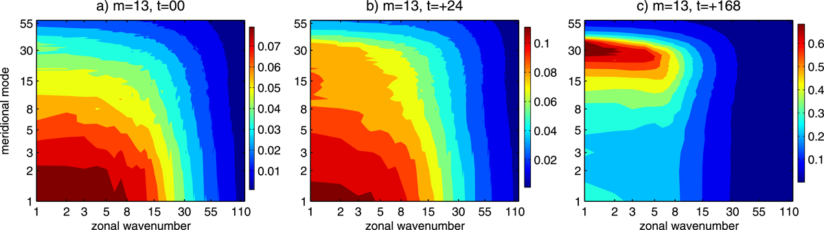
Figure 4.
As in Fig. 3 but for the balanced vertical mode with the equivalent depth around 25 m.
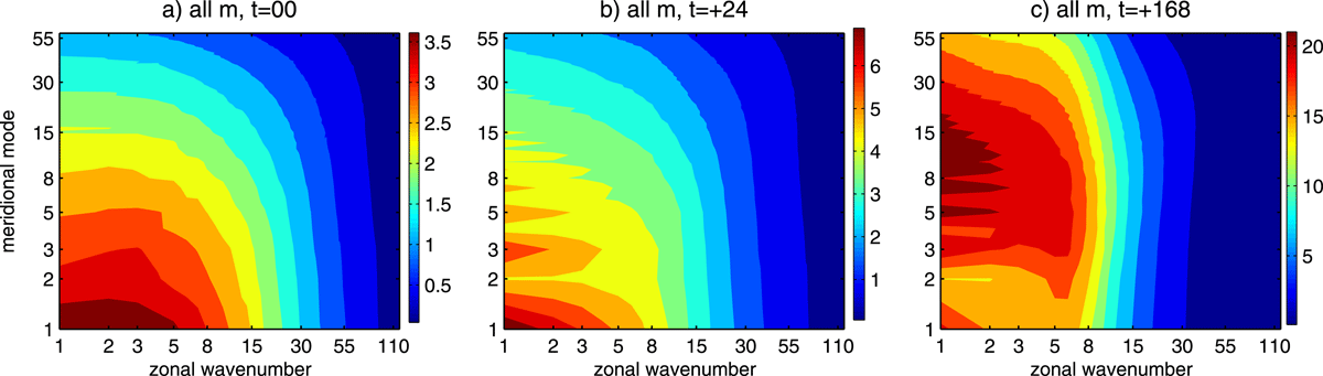
Figure 5.
As in Fig. 3 but the sum of the balanced spread in all vertical modes.
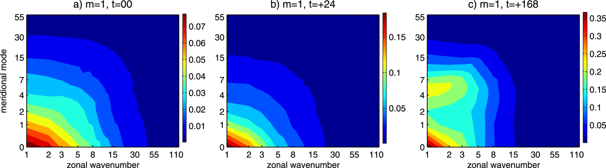
Figure 6.
As in Fig. 3 but for the EIG spread.
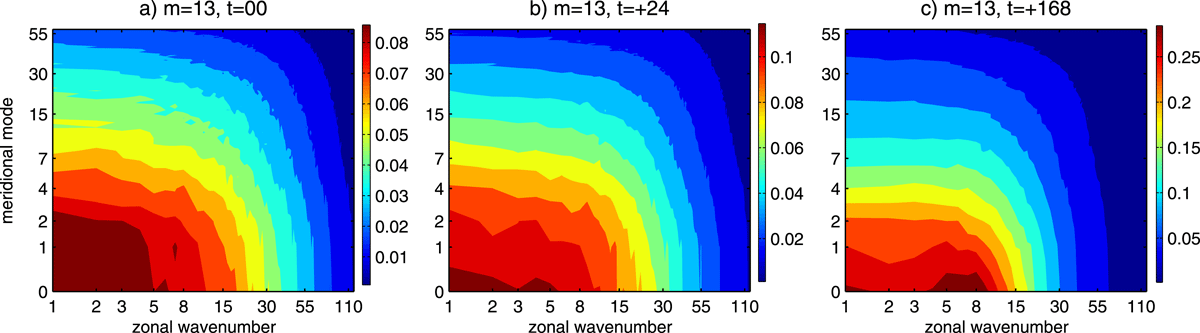
Figure 7.
As in Fig. 4 but for the EIG spread.
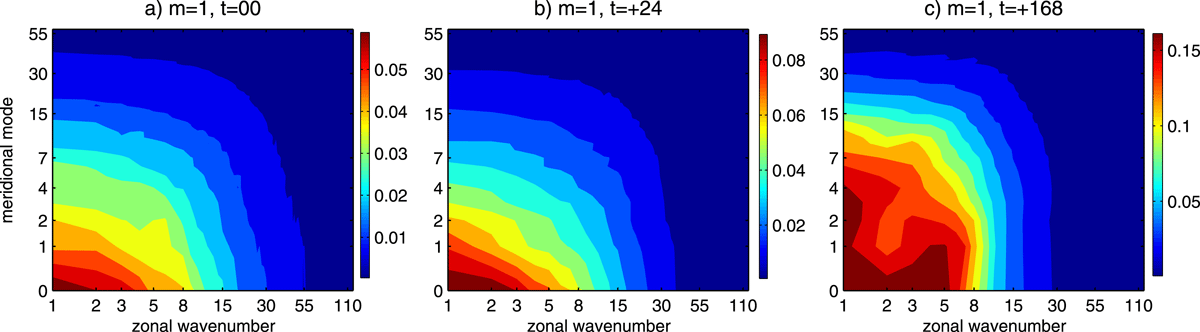
Figure 8.
As in Fig. 3 but for the WIG spread.
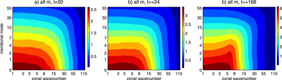
Figure 9.
As in Fig. 5 but for the WIG spread.
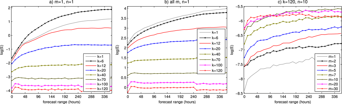
Figure 10.
The growth of estimated forecast errors in selected meridional modes and zonal scales as a function of the zonal wavenumber and vertical mode (as specified in the legend). (a) meridional mode and vertical mode , (b) meridional mode and all vertical modes integrated and (c) meridional mode and zonal wavenumber . The presented quantity is integrated over individual modes as specified in the legends.
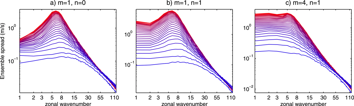
Figure 11.
The growth of ensemble spread in selected balanced modes as a function of the zonal wavenumber. The bottom curve in each panel shows spread at the initial time whereas every next curve applies to 12-h longer forecasts. (a) meridional mode and vertical mode , (b) meridional mode and vertical mode , and (c) meridional mode and vertical mode .
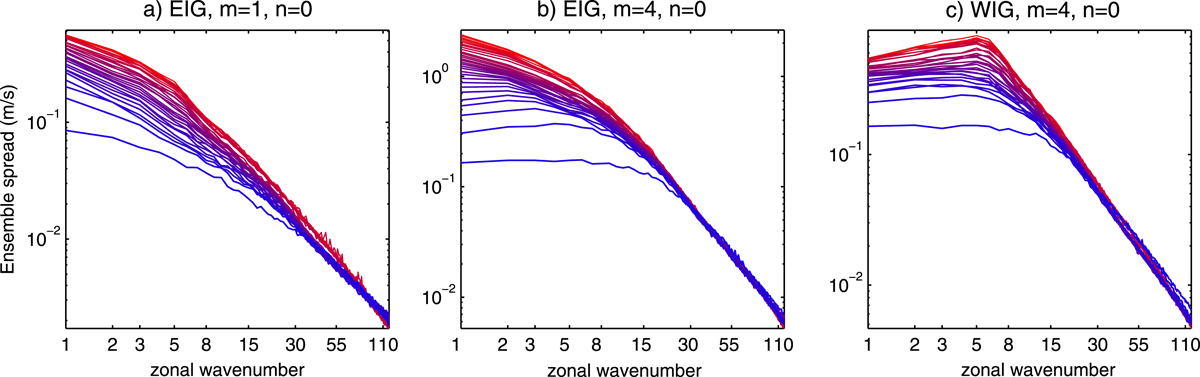
Figure 12.
As in Fig. 11 but for the IG modes. (a) EIG mode with meridional index and the first vertical mode , (b) EIG mode with meridional index and vertical mode , and (c) WIG meridional mode and vertical mode .
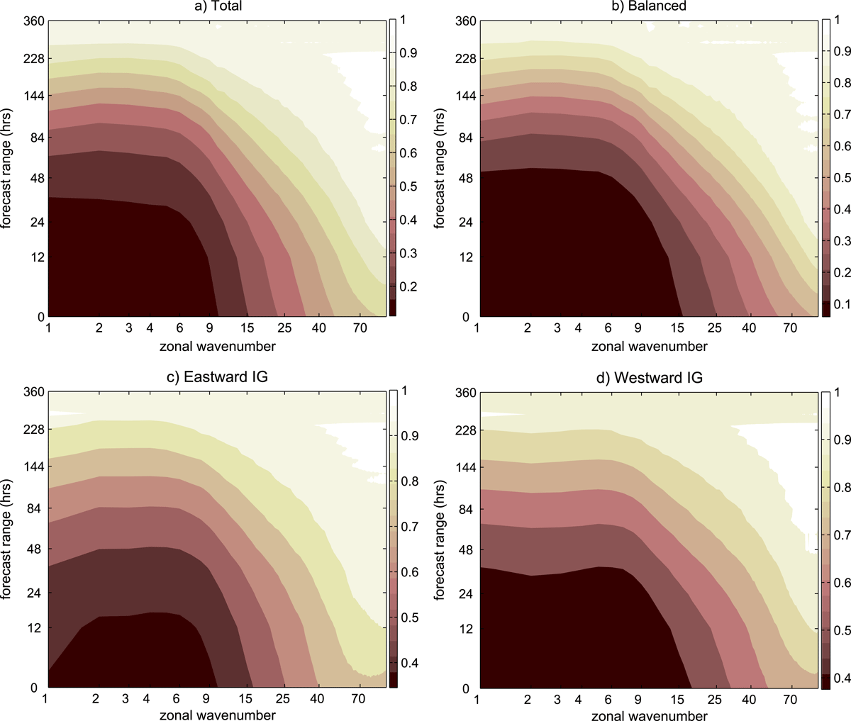
Figure 13.
Ensemble spread as a function of the zonal wavenumber normalized by the spread at the forecast range 360 h in the same zonal wavenumber. (a) Total spread, h), (b) balanced spread, h), (c) eastward-propagating inertio-gravity spread, h) and (d) westward-propagating inertio-gravity spread, h). The axes are logarithmic.
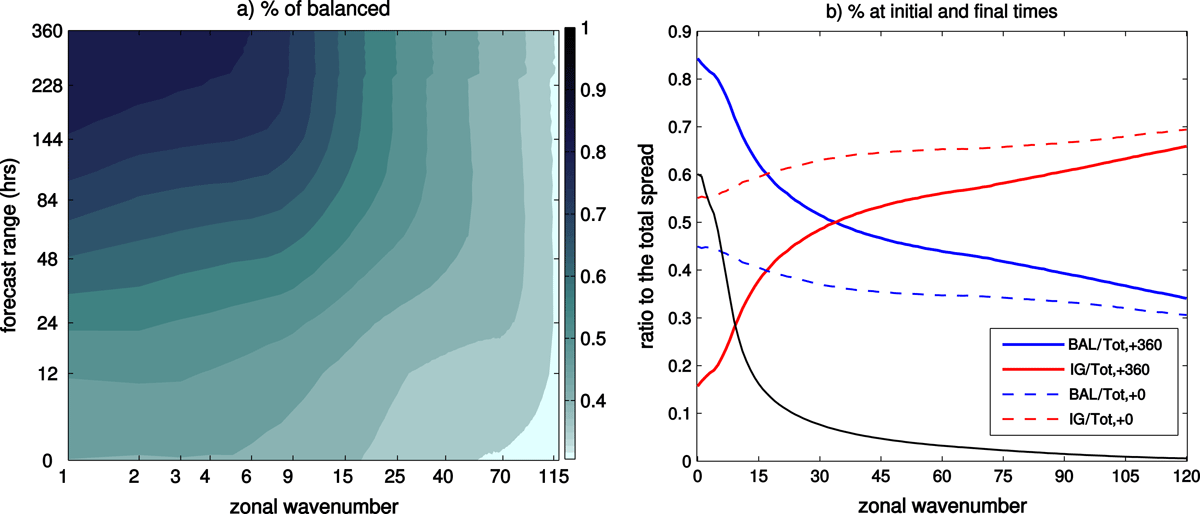
Figure 14.
(a) Balanced ensemble spread as a function of the zonal wavenumber normalized by the total spread at the same forecast range and zonal wavenumber, , (b) Portion of the global spread at initial time and 15-day range in balanced and IG components in each zonal wavenumber. Different colour lines are specified in legend. Blue lines are (dashed) and (full) , red lines represent (dashed) and (full) . Black line corresponds to the portion of the total spread in each zonal wavenumber at 2-week range multiplied by 10.
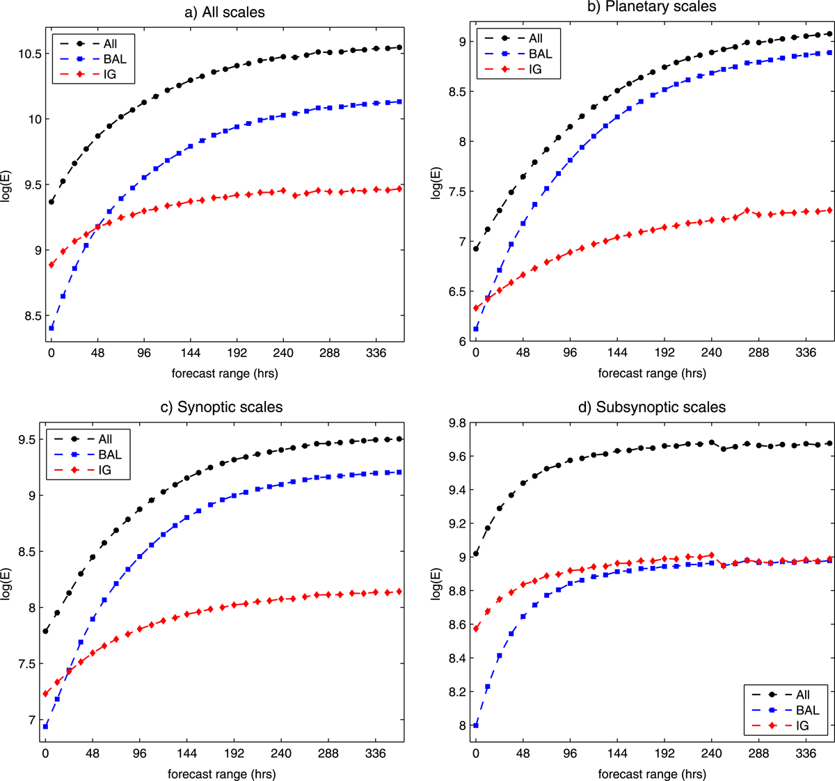
Figure 15.
The scale-dependent growth of estimated forecast errors in the balanced and inertio-gravity regimes. The presented quality is the global error integrated over (a) all scales (, , ), (b) planetary scales (, , ), (c) synoptic scale (, , ) and (d) subsynoptic scales (, , ).