
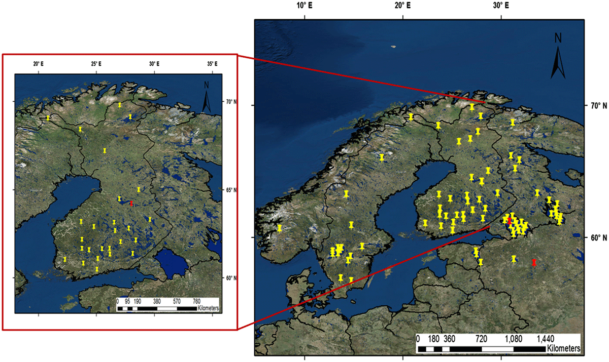
Figure 1.
Location of the selected MODIS pixels (the main fugure) and SYKE measurement points (in the frame) over the lakes used to calculate the autocorrelation function and in HIRLAM data assimilation experiments over the Northern Europe. Locations of three passive observations, which are central in the discussion in Section 4 are shown in red. The list of all passive observations is presented in Table 3.
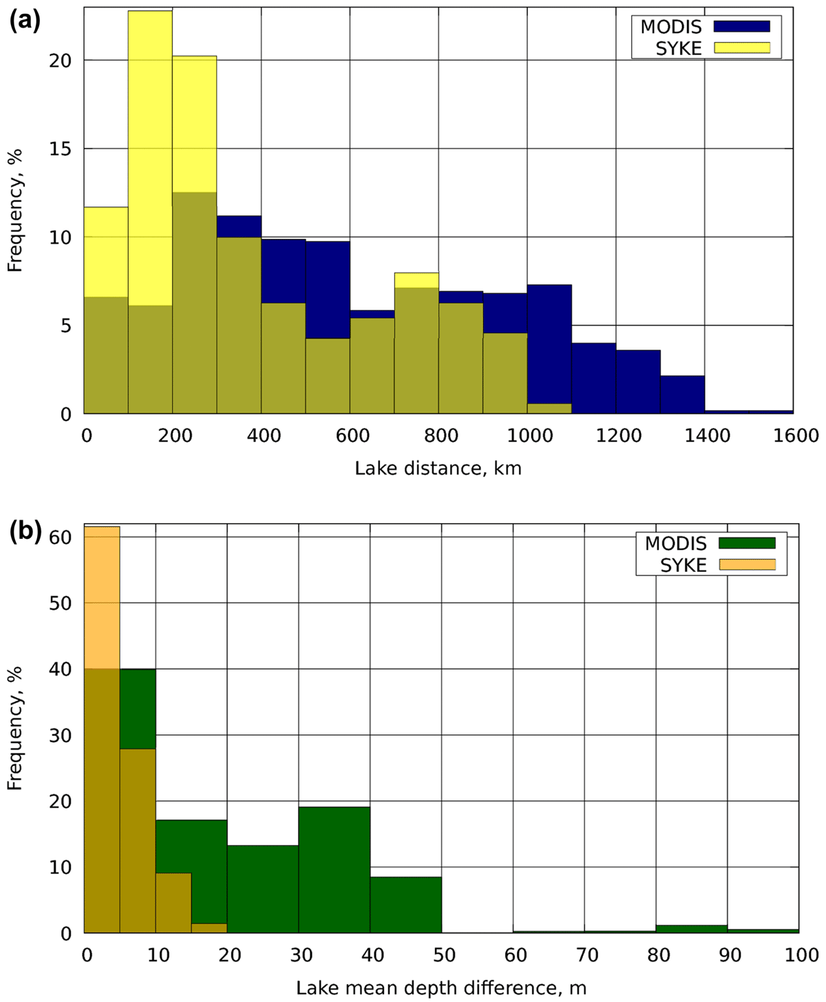
Figure 2.
Distribution (frequency in %) of distance (left) and depth difference (right) between the pairs of SYKE lakes (351 pairs) and MODIS pixels (2401 pairs).
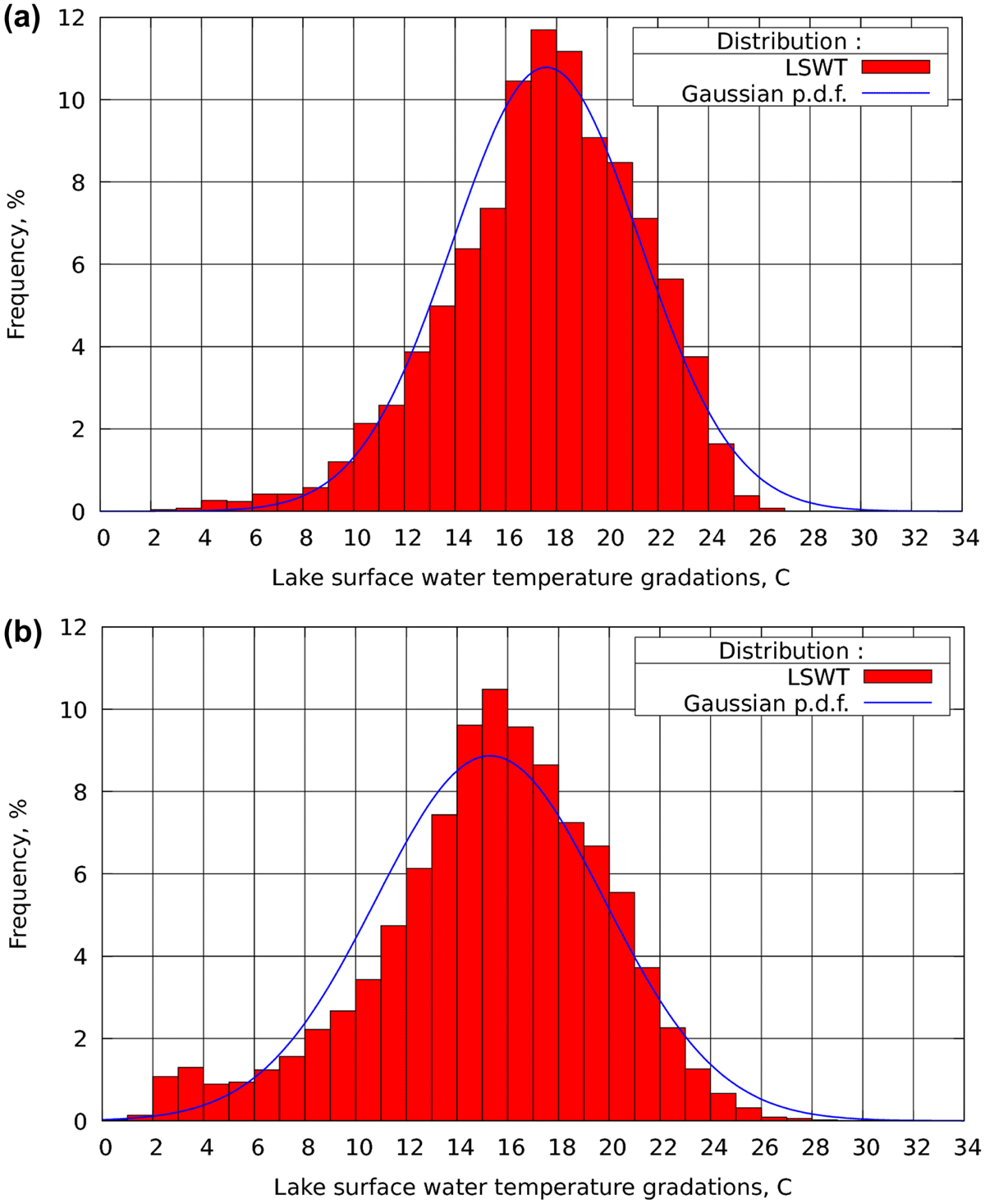
Figure 3.
Frequency distribution (%, red bars) of LSWT from data for the period of JJA 2010-2014 and the Gaussian distribution (%, blue lines) with the mean values and standard deviations from Table 1: left) SYKE, right) MODIS.
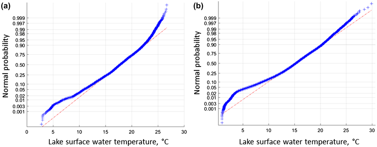
Figure 4.
Normal probability plots of (a) SYKE LWT and (b) MODIS LSWT observations (C) for JJA 2010–2014. Deviation of points from the straight line suggests departures from normality. Here, the blue crosses fall approximately on the red lines, which indicates normal distribution of the data.
Table 1.
Statistical properties of the observed LSWT for 2010–2014 June-July–August. N is the number of observations.
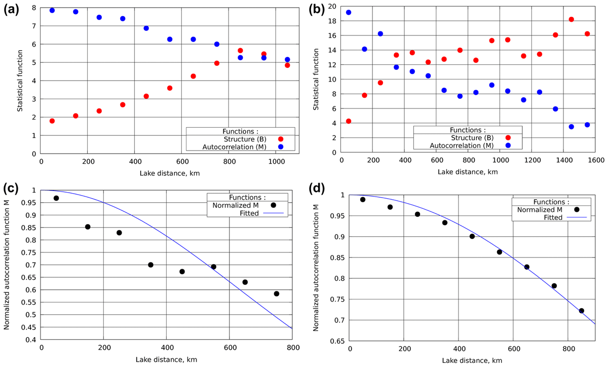
Figure 5.
Upper panel: the calculated structure (Equation (A4), red dots) and autocorrelation (Equation (A6), blue dots) functions depending on distance based on observations from SYKE (left) and MODIS (right). Lower panel: the normalized autocorrelation function (Equation (A8), black dots) with the exponential approximation (Equation (A10), blue line) based on observations from SYKE (left) and MODIS (right). Parameters of exponential function are given in the text. On the upper panel, note the right limit of x-axis: 1100 km for SYKE and 1600 km for MODIS, and the upper limit of y-axis: 8 C for SYKE and 20 C for MODIS.
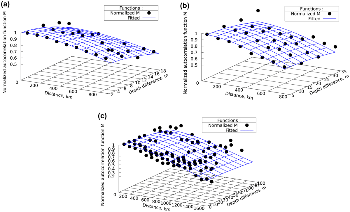
Figure 6.
Normalized autocorrelation function depending on distance and depth difference (black dots) with an exponential approximation (blue grid): (a) SYKE, (b) MODIS, (c) MODIS all cases. The influence radiuses are discussed in the text.
Table 2.
The autocorrelation function of LSWT depending on distance, estimated from SYKE and MODIS data, and the confidence of estimates. N is the number of observations. For notation, see Equation (A12).
Table 3.
List of independent (passive) observations for HIRLAM experiment validation.
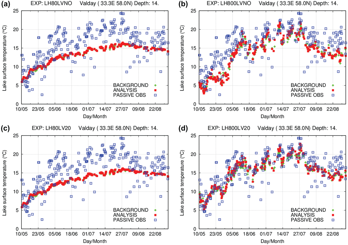
Figure 7.
Evolution of the LSWT on Lake Valday for the period of May–August 2011 in the experiments (a) LH80LVNO, (b) LH800LVNO, (c) LH80LV20 and (d) LH800LV20: background (green marks), analysed (red) and observed (passive MODIS measurements at this point, blue) values.
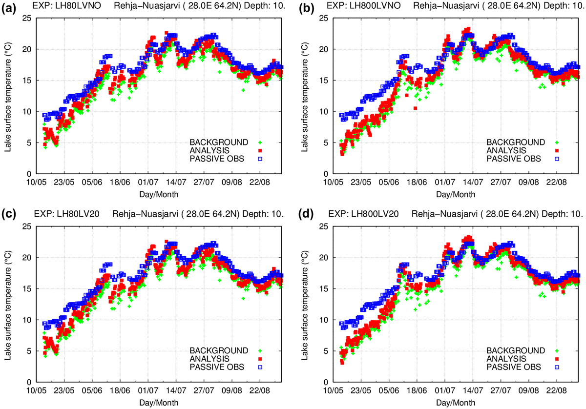
Figure 8.
Notation as for Fig. 7, but for Lake Rehja-Nuasjärvi and SYKE observations.
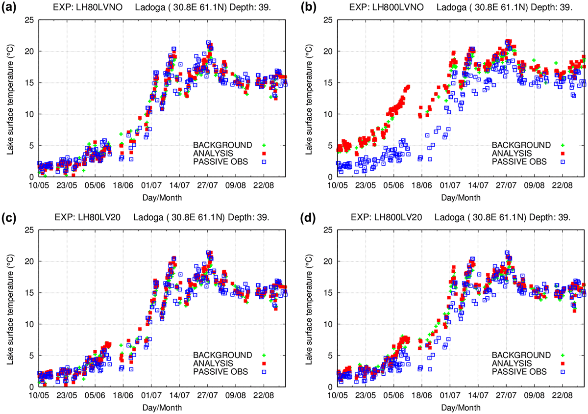
Figure 9.
Notation as for Fig. 7, but for Lake Ladoga.