
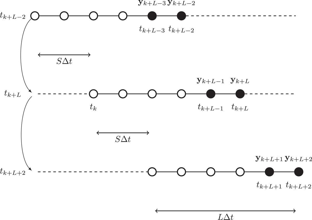
Figure 1.
Typical cycling of the smoothers considered in this study, in the specific case where and , in units of , the time interval between two updates. The method performs a smoothing update throughout the window but only assimilates the newest observations vectors (that have not been already assimilated) marked by black dots. Note that the time index of the dates and the observations are absolute for this schematic, not relative.
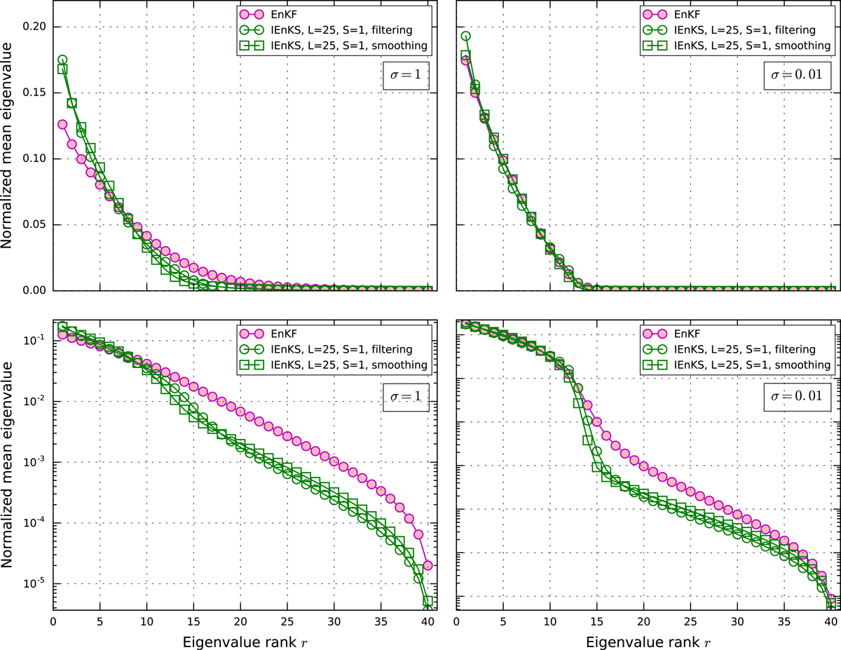
Figure 2.
Mean eigenvalues of the analysis error covariance matrix normalized by the total variance, in linear (top panels) and in logarithmic scale (bottom panels) for the EnKF and the IEnKS with and , and for an observation error standard deviation (left panels) and (right panels). For the IEnKS, the average normalized spectra of both (smoothing covariances) and (filtering covariances) are shown. The set-up is , , and .
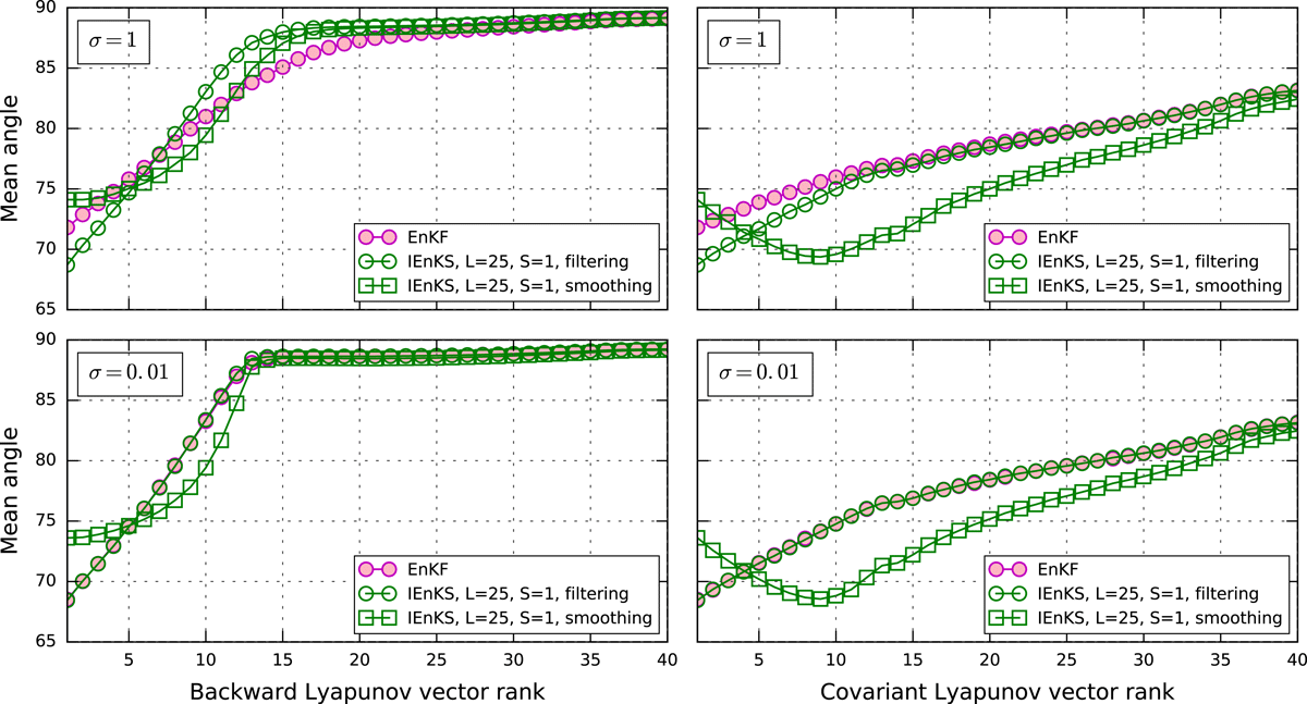
Figure 3.
Time- and ensemble-averaged angle (in degree) defined by Equation (54), of the anomalies of the ensemble onto each of the backward (left panels) and covariant (right panels) Lyapunov vectors for the EnKF and the IEnKS with and , and for an observation error standard deviation (upper panels) and (lower panels). For the IEnKS, the average normalized spectra of both (smoothing covariances) and (filtering covariances) are shown. The se-tup is , , and .
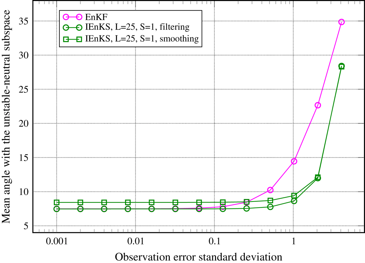
Figure 4.
Time- and ensemble-averaged angle (in degree) from Equation (55), between an anomaly from the EnKF ensemble and from the IEnKS ensemble (, ) and the unstable–neutral subspace, when the observation error standard deviation is varied from to 4. The set-up is , , and .
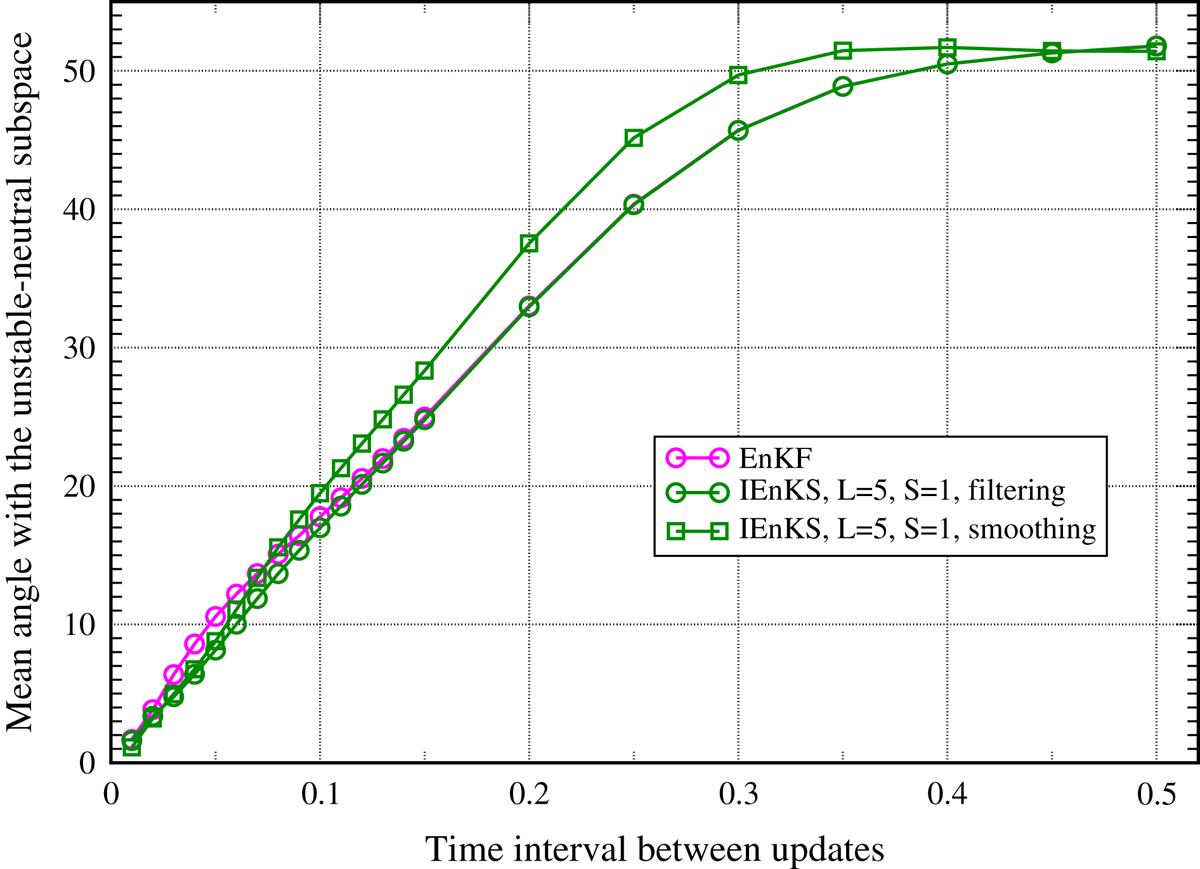
Figure 5.
Time- and ensemble-averaged angle (in degree) from Equation (55), between an anomaly from the EnKF and IEnKS (, ) ensembles and the unstable–neutral subspace, when the time interval between updates is varied from to . The se-tup is , with and .
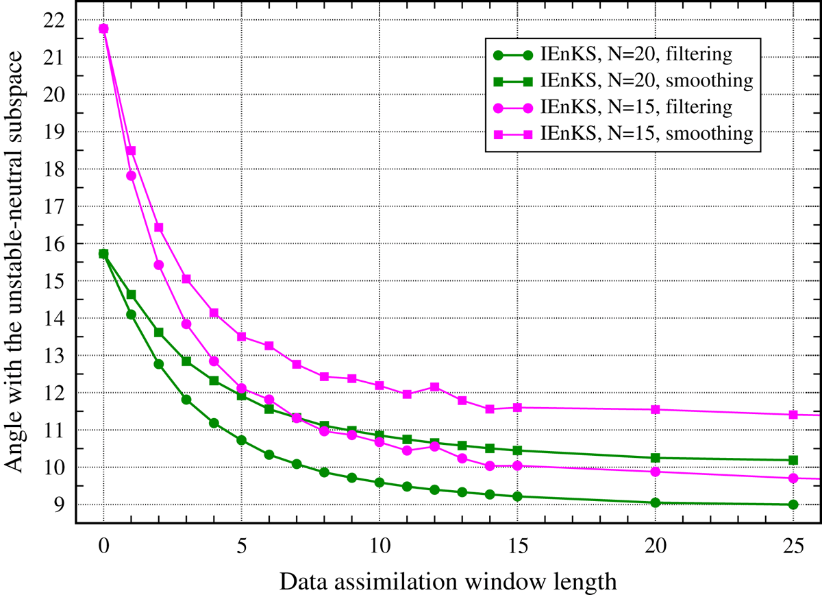
Figure 6.
Time- and ensemble-averaged angle (in degree) from Equation (55), between an anomaly from the IEnKS ensemble and the unstable–neutral subspace, when the DAW length is varied from (corresponding to the EnKF) to , and . The set-up is , and .
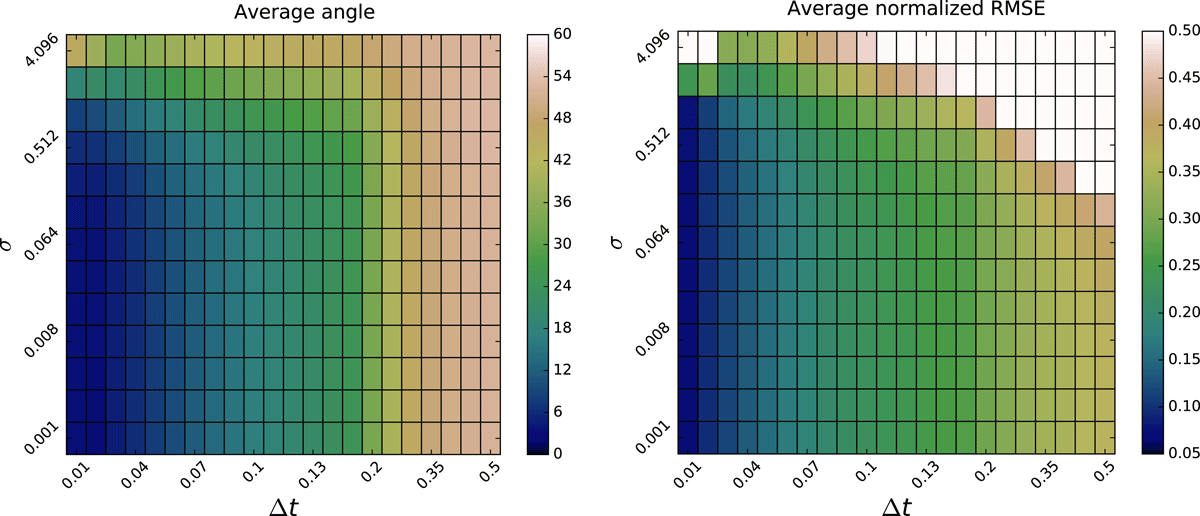
Figure 7.
Time- and ensemble-averaged angle from Equation (55) (left panel, shadow colours in degree) between an anomaly of the EnKF and the unstable–neutral subspace, and the EnKF RMSE normalized by (right panel, shadow colours), on the plane . The set-up is , and .
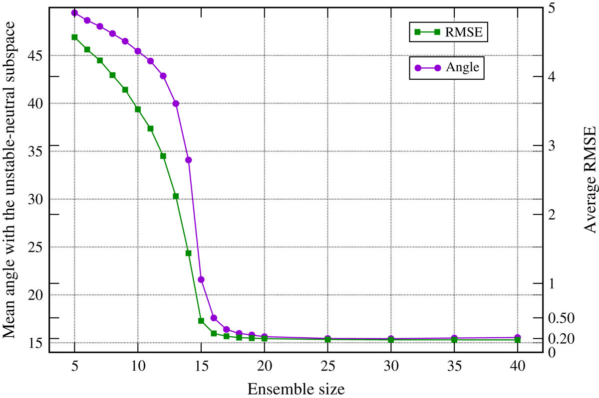
Figure 8.
Time- and ensemble-averaged angle (in degree) between an anomaly from the EnKF ensemble and the unstable–neutral subspace as a function of the ensemble size N (left Oy axis) and corresponding time-averaged RMSE of the EnKF (right Oy axis). The set-up is , , and .
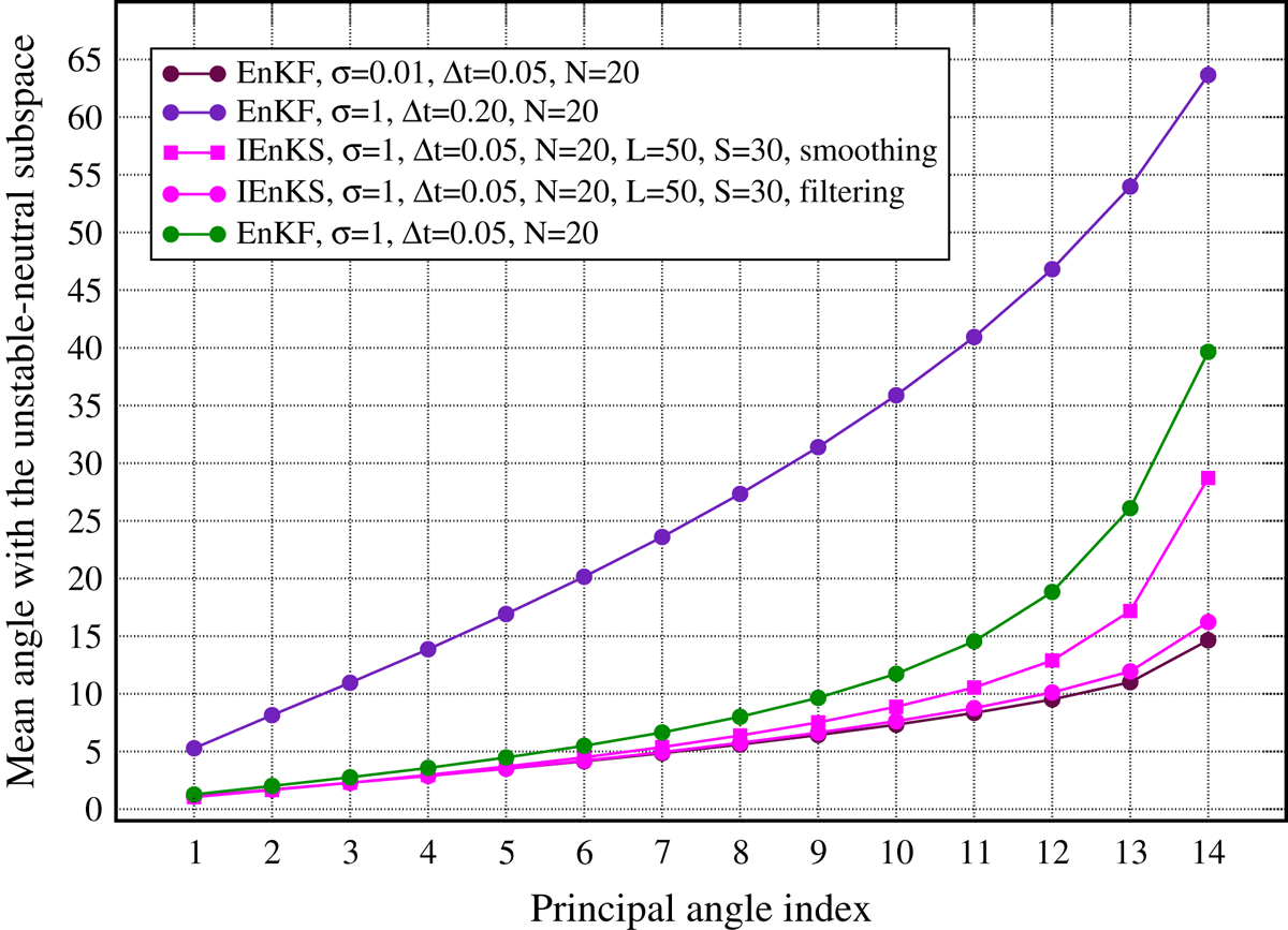
Figure 9.
Time-averaged principal angle (in degree) between the anomaly simplex (see text) and the unstable–neutral subspace, as a function of its index for several EnKF/IEnKS configurations (see legend).
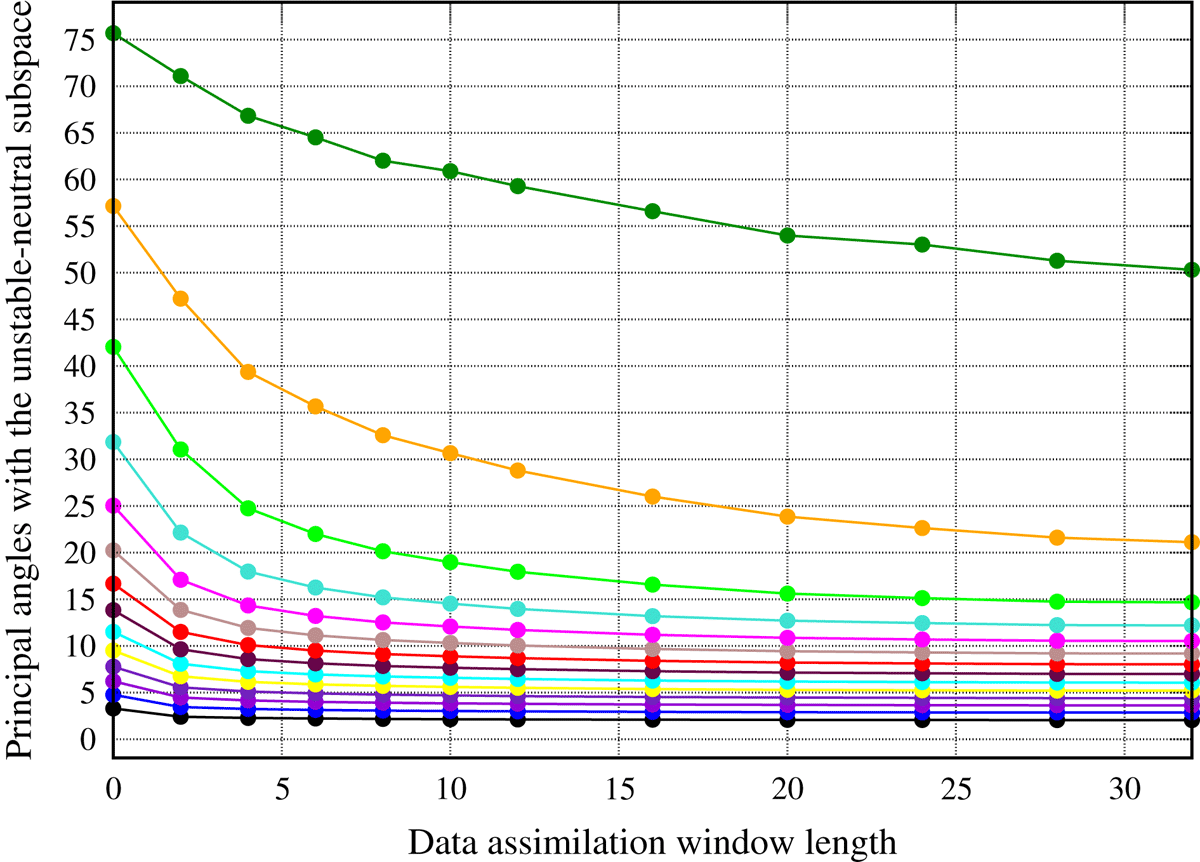
Figure 10.
The 14 time-averaged principal angles (in degree) between the IEnKS anomaly subspace of the smoothing analysis and the unstable–neutral subspace, as a function of the DAW length. The set-up is , , , and .