
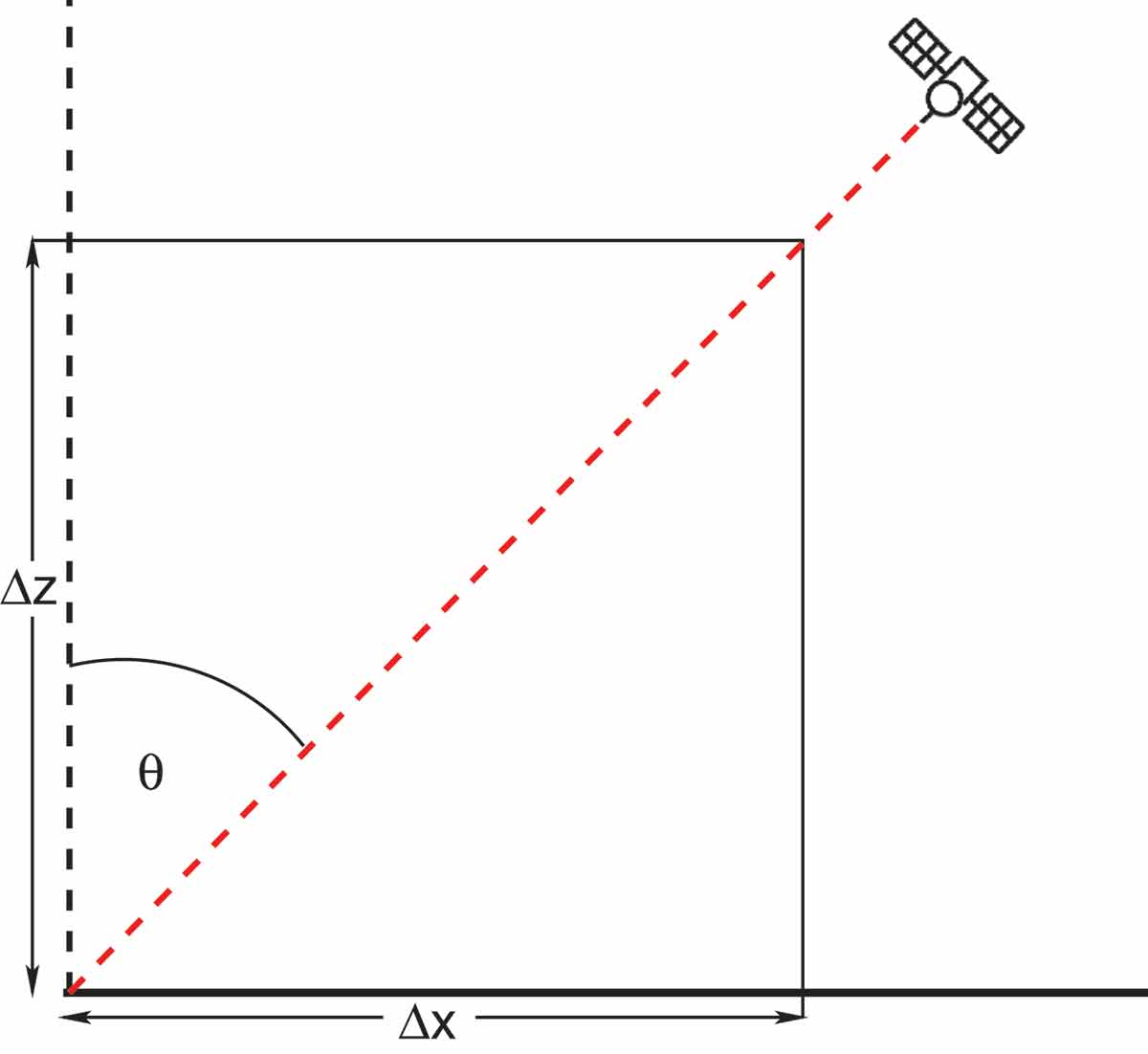
Figure 1.
Schematic illustration of the satellite viewing geometry, viewing a location on Earth with a zenith angle of along a slanted path through the atmosphere (red). The vertical profile currently used for radiative transfer calculations is indicated in black.
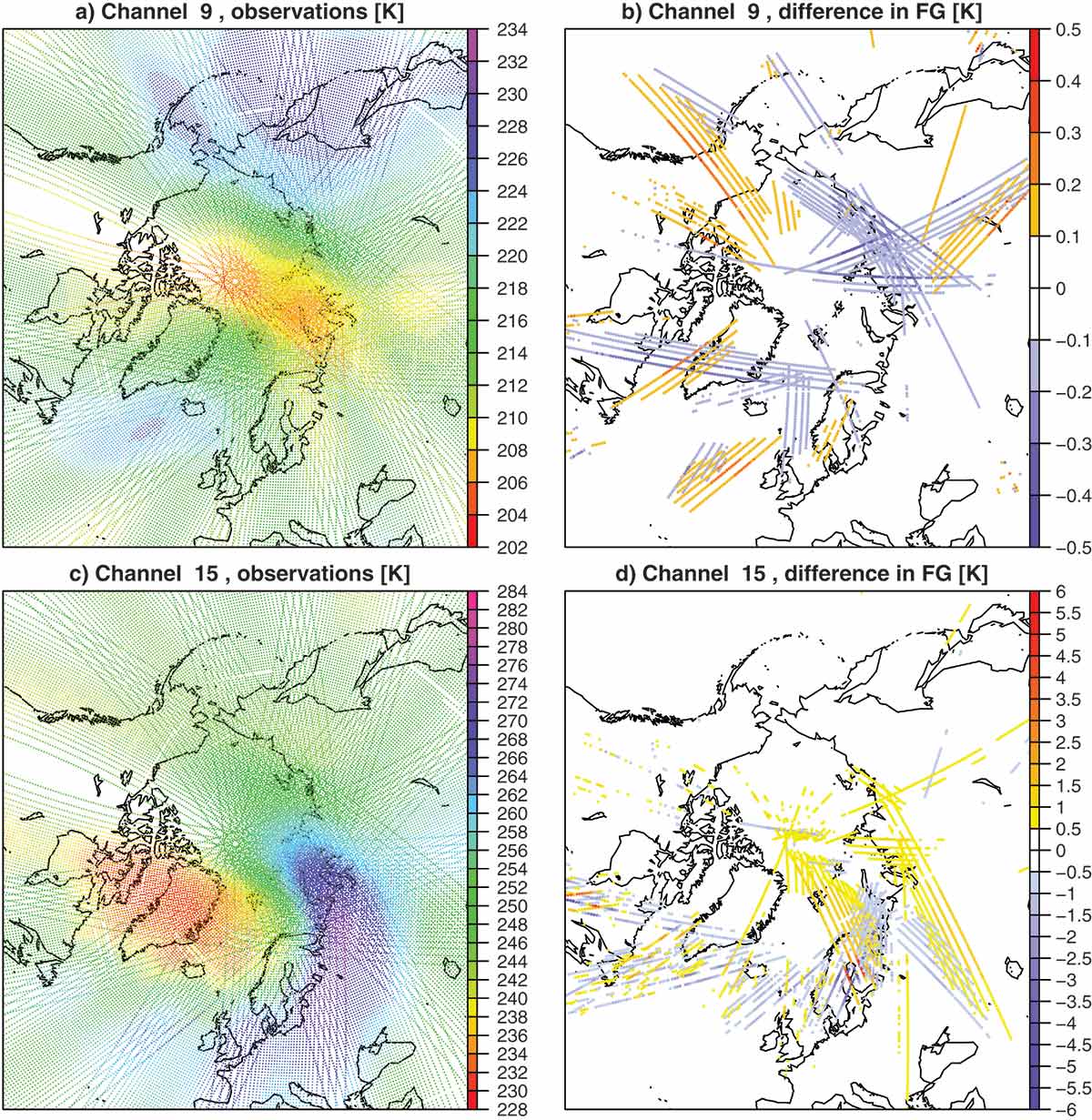
Figure 2.
(a) Observed brightness temperatures [K] for ATMS channel 9 for a 12-hour period around 25 January 2015 00UTC. (b) Difference in the radiative transfer simulations from short range forecasts with and without taking the slant-path effect into account, for the observations shown in a). Note that only differences with an absolute value larger than 0.1 K are shown. (c) As a), but for channel 15 of ATMS. (d) As (b), but for the observations shown in (c). Note that only differences with an absolute value larger than 0.5 K are shown here.
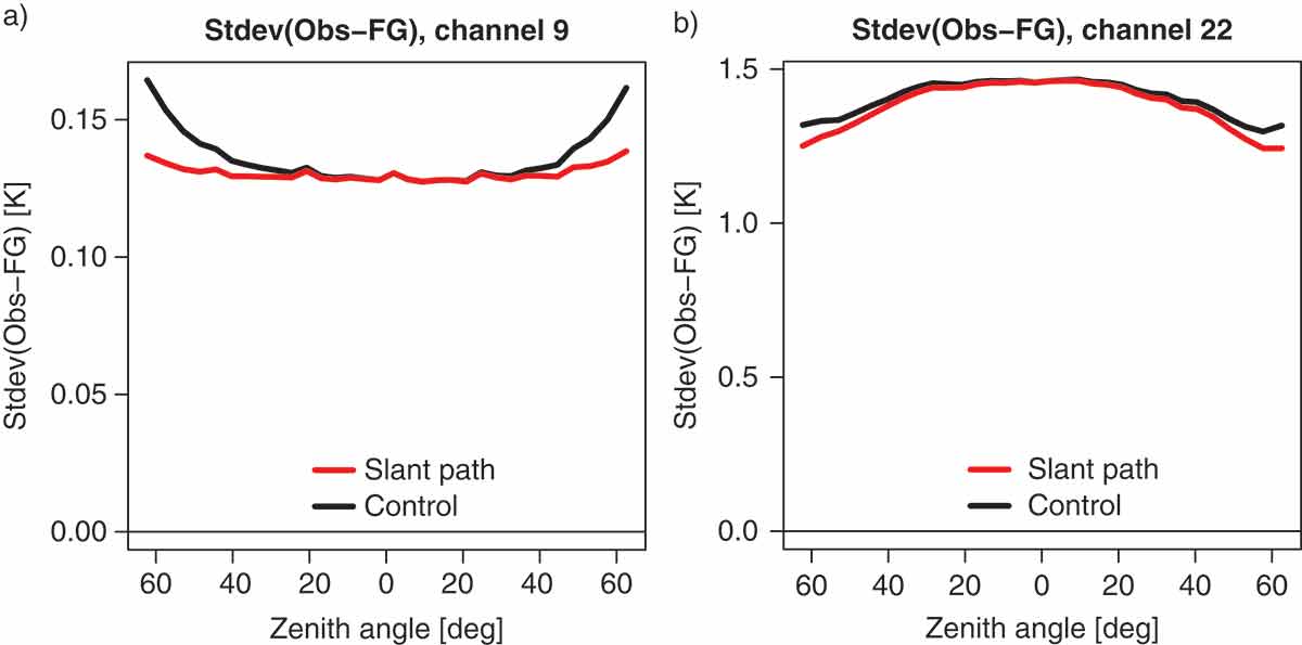
Figure 3.
(a) Standard deviations of differences between observations and short-range forecast equivalents for channel 9 of ATMS as a function of the scan position (labelled here with the average satellite zenith angle). Black indicates the conventional treatment, red indicates statistics for calculations that take the slant-path geometry into account. The statistics cover the period 25 January to 24 February 2015, and are based on data over sea after cloud/rain screening. Biases have been removed based on bias corrections obtained from the underlying assimilation experiment that uses the conventional radiative transfer simulations. (b) As a), but for channel 22 of ATMS, the highest peaking humidity sounding channel.
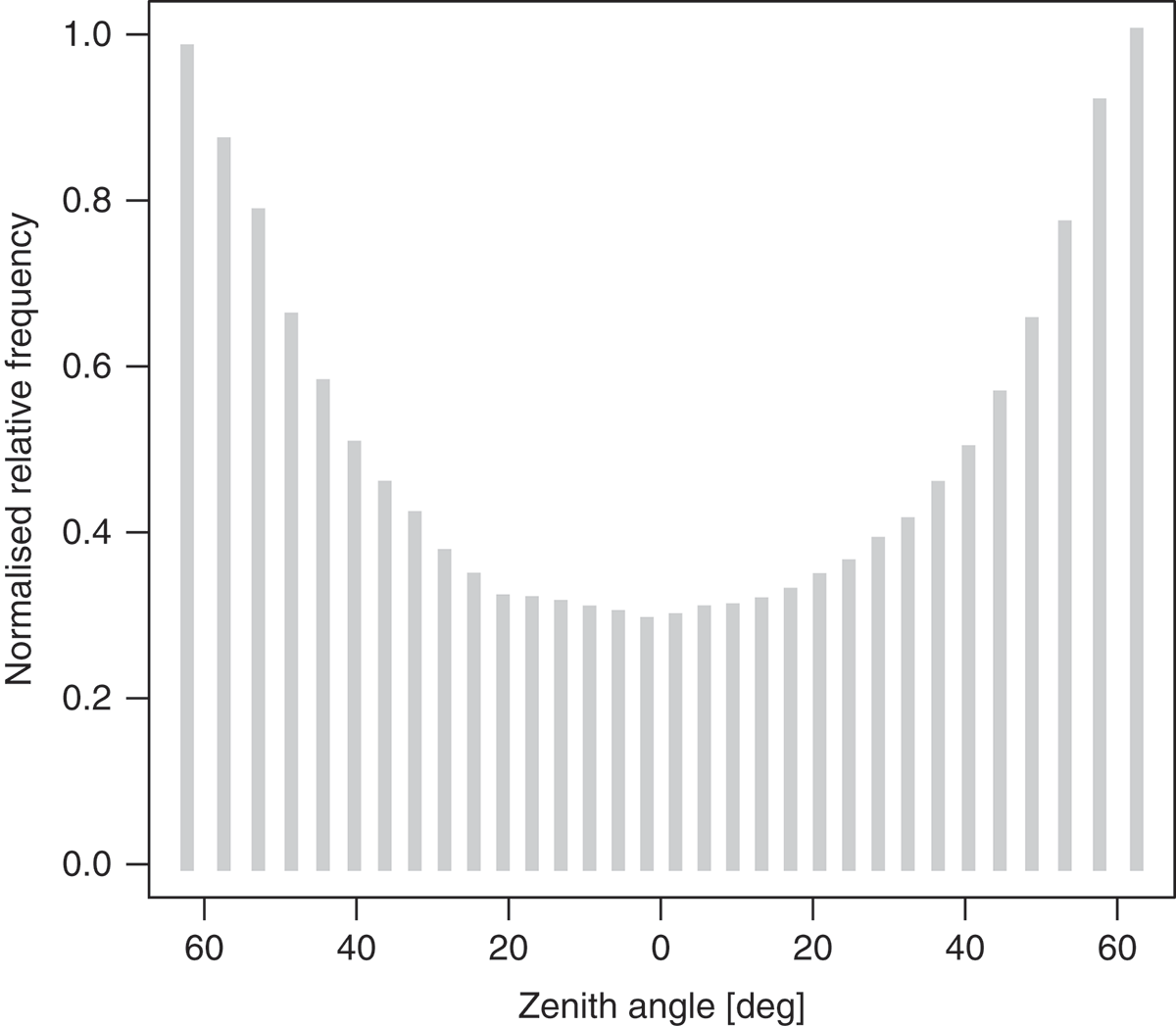
Figure 4.
Normalised relative frequency of observations after geophysical quality control and after spatial thinning as a function of scan-position (labelled here by average zenith angle) for ATMS. The normalised relative frequency shown is the number of observations normalised by the maximum number of observations for any scan position.
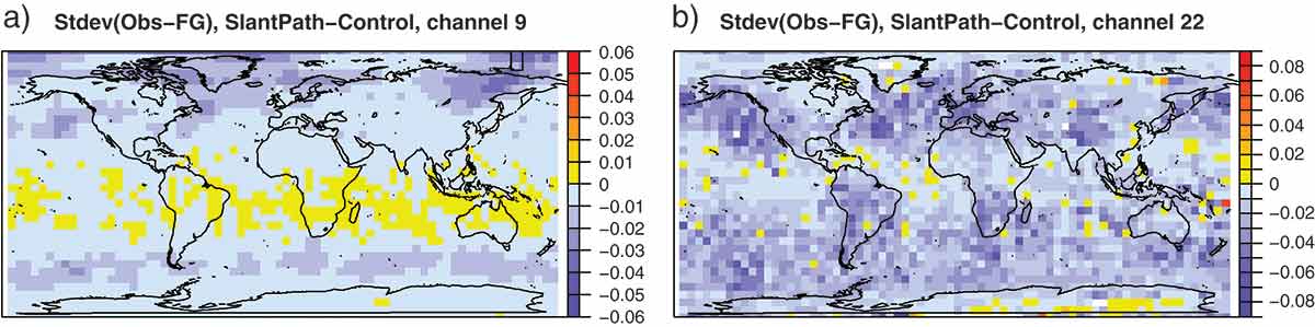
Figure 5.
(a) Maps of the difference in the standard deviations of the departures [K] for channel 9 of ATMS between taking the slant-path geometry into account and neglecting the slant-path geometry. Negative values indicate a reduction in the standard deviations from taking the slant-path geometry into account. Statistics are based on simulations from the same short-range forecasts, covering the period 25 January to 24 February 2015, after geophysical quality control. Biases have been removed based on bias corrections obtained from the underlying assimilation experiment that uses the conventional radiative transfer simulations. (b) As (a), but for channel 22.
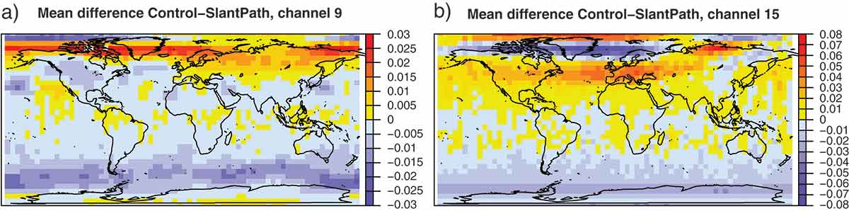
Figure 6.
(a) Maps of the mean difference [K] between neglecting the slant-path geometry and taking it into account in the simulations from short-range forecasts for channel 9 of ATMS on S-NPP. Statistics are based on simulations from the same short-range forecasts, covering the period 25 January to 24 February 2015, after geophysical quality control applied to the underlying observations. (b) As (a), but for channel 22.
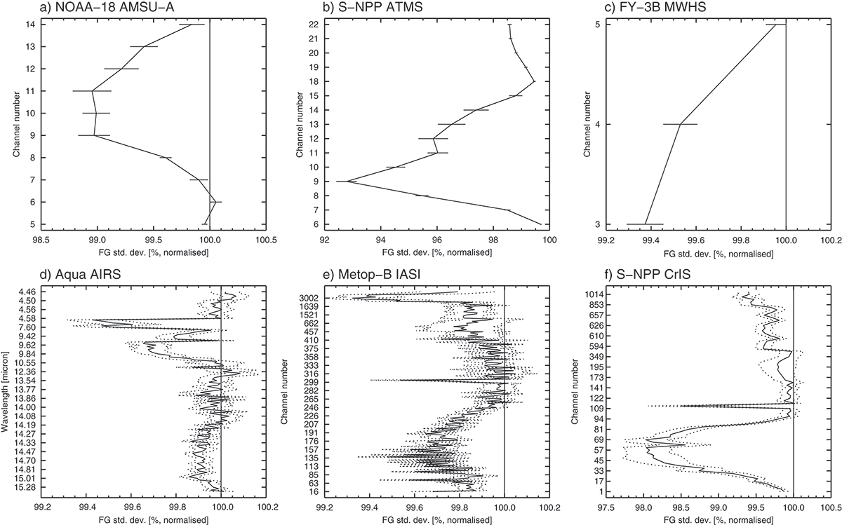
Figure 7.
Standard deviation of differences between observations and simulations that take the slant-path geometry into account, normalised by equivalent values obtained with simulations that ignore the slant-path geometry. Values below 100% indicate smaller standard deviations when the slant-path geometry is taken into account. Horizontal bars indicate 95% significance intervals. Statistics are based on data covering the period 25 January to 24 February 2015, after quality control and thinning and after applying bias correction. The six panels show: (a) Statistics for AMSU-A on NOAA-18, (b) ATMS on S-NPP, (c) MWHS on FY-3B, (d) AIRS on Aqua, (e) IASI on Metop-B, and (f) CrIS on S-NPP.
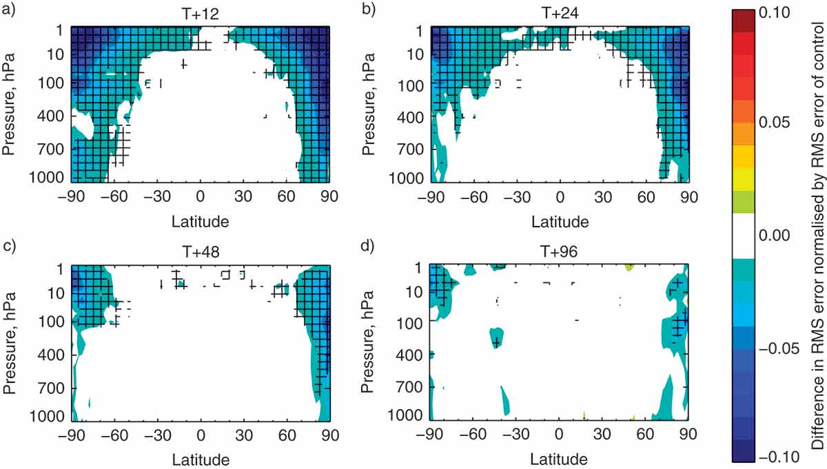
Figure 8.
(a) Zonal means of normalised differences in the root mean squared vector wind analysis increments between the SlantPath experiment and the Control. Blue indicates a reduction in the standard deviation of the increments in the SlantPath experiment compared to the Control. Cross-hatching marks statistical significance at the 95% confidence level. (b) As (a), but for the root mean squared vector error of the 24-hour forecast verified against its own analysis. (c) As (b), but for the 2-day forecast. (d) As (a), but for the 4-day forecast. All statistics cover approximately 8 months over the two seasons combined, with a total of 430 to 468 samples.
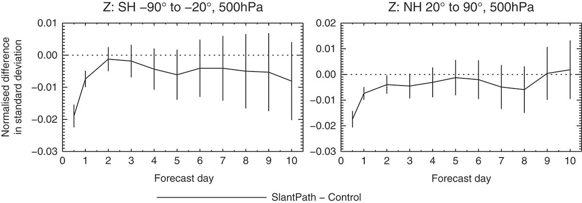
Figure 9.
Normalised difference in the standard deviation of forecast errors in the 500 hPa geopotential as verified against each experiment’s own analysis for the Southern Hemisphere extra-tropics (left) and the Northern Hemisphere extra-tropics (right). Vertical bars indicate 95% significance intervals.