
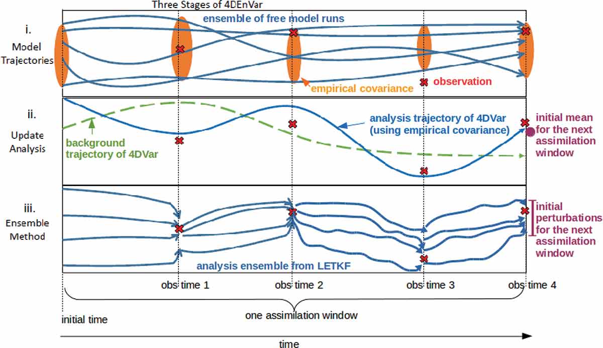
Fig. 1.
Schematic depicting the three stage process of 4DEnVar. In part i an ensemble of ‘free’ (DA-less) trajectories of the model is run for the length of the assimilation window. In part ii the 4DVar minimisation process is performed using 4-dimensional cross-time covariances instead of tangent linear and adjoint models. In part iii an LETKS is run to the end of the assimilation window to create new initial conditions for the next window. The mean of this LETKS is replaced by the solution of 4DEnVar, considered to be more accurate.
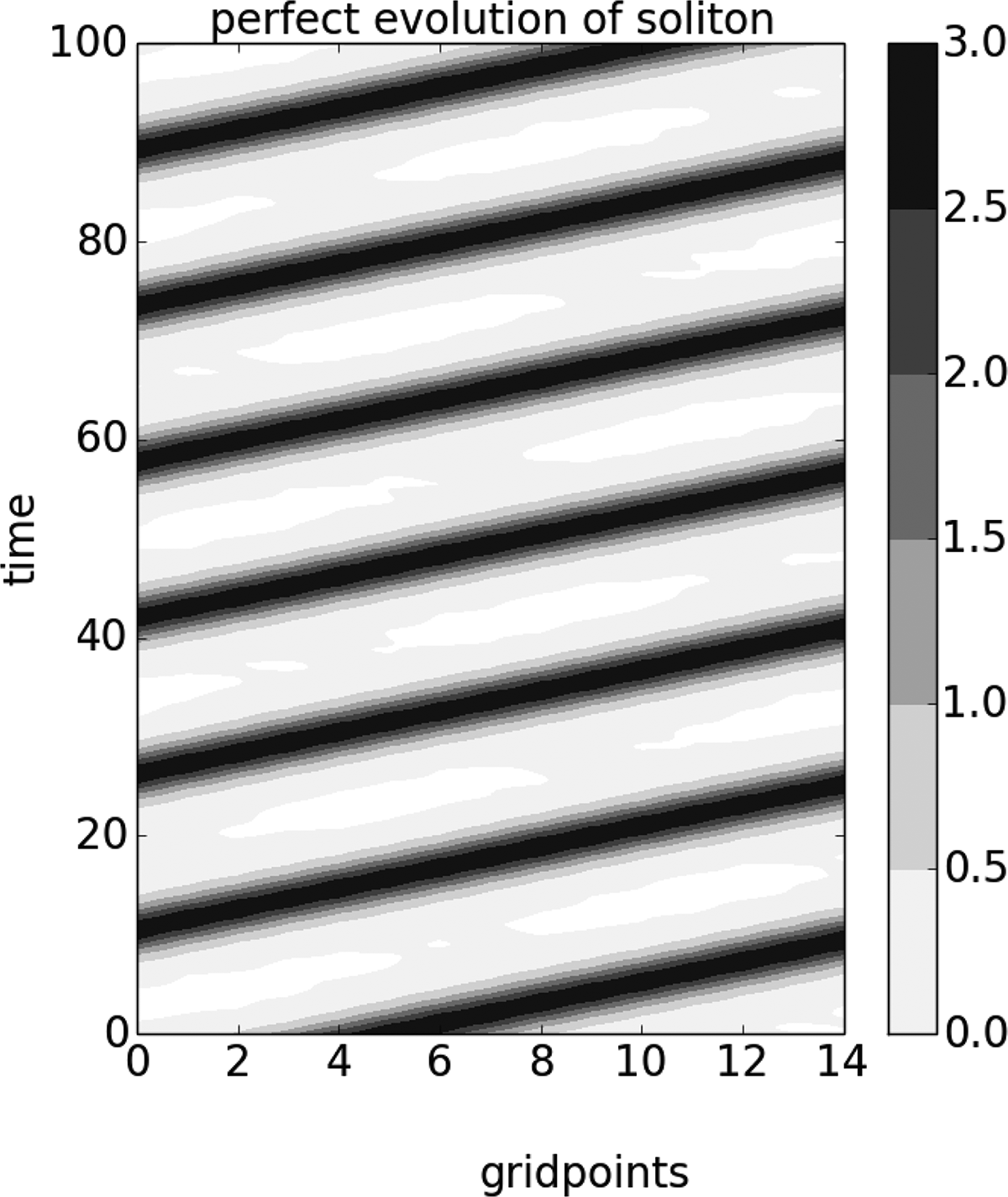
Fig. 2.
Hovmoller plot showing the perfect evolution of a soliton produced by a numerical integration of the KdV equation over a periodical domain of 15 grid points.
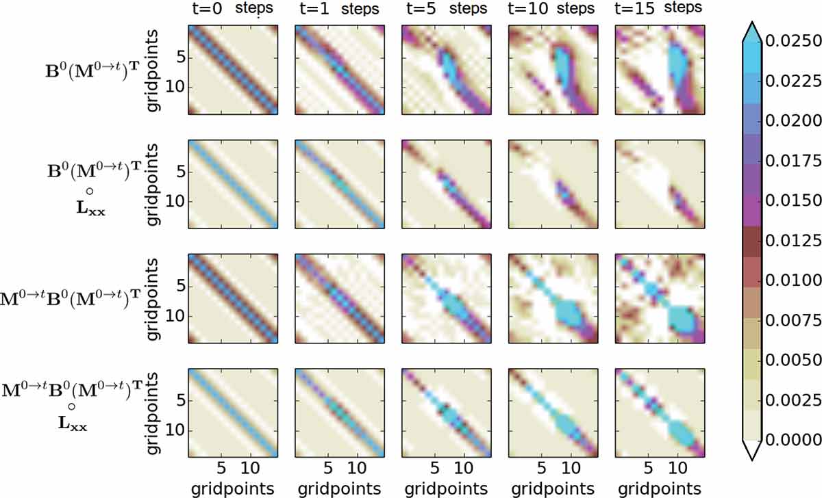
Fig. 3.
Analytical evolution of the covariance and cross-time covariance for the KdV model for different times (columns). The horizontal and vertical axes of each panel are the grid point locations. The first row shows and the second shows its localised version. The third row shows and the fourth shows its localised version.
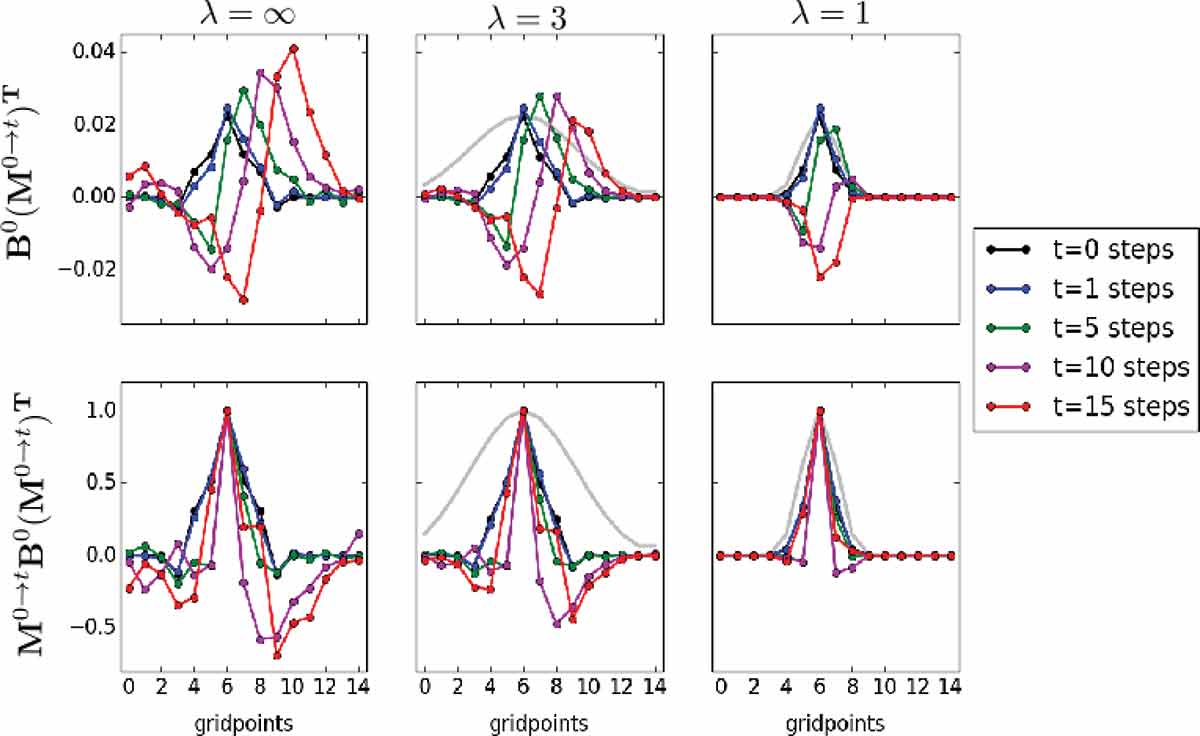
Fig. 4.
Elements of the 6th row of the matrices (top row) and (bottom row), for different times (different colors). The first column shows the unaltered elements, while the middle and right columns show these elements after being localised using Gaspari-Cohn functions of different half-widths (gray lines).
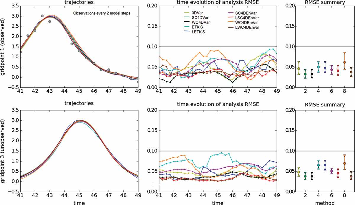
Fig. 5.
Using different DA methods in the KdV model for an observation period of 2 model steps. The left panels show the time evolution of the nature run (black line) and the analysis trajectories generated by different DA methods (color lines). The top row shows the case of grid point 1 (observed variable, observations are represented with gray circles), while the bottom row shows the case of grid point 3 (unobserved variable). The middle panels show the time evolution of the analysis RMSE. The top panel corresponds to observed variables, while the bottom panel corresponds to unobserved variables. For both cases, the horizontal gray line is the standard deviation of the observational error. The right panels show summary statistics for observed (top panel) and unobserved variables (bottom panel). We show intervals containing the first, second (median) and third quartiles of the analysis RMSE distribution in time.
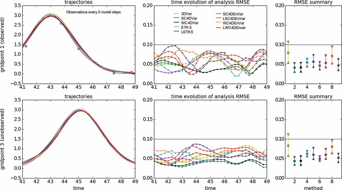
Fig. 6.
Same as Fig. 5 but with an observational period of 5 model time steps.
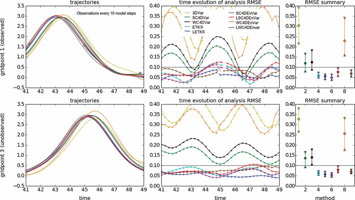
Fig. 7.
Same as Fig. 5 but with an observational period of 10 model time steps.
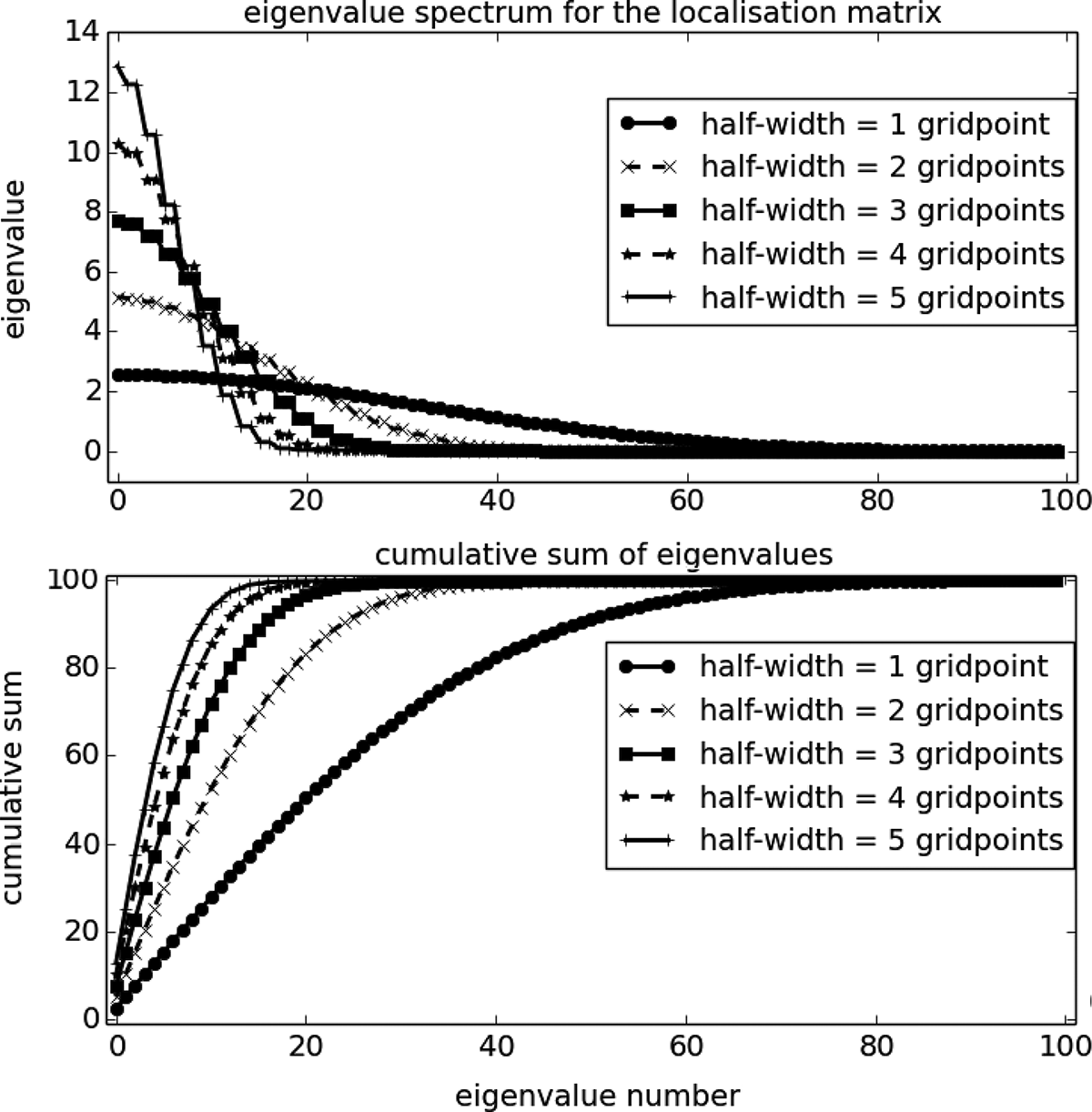
Fig. 8.
Eigenvalue spectrum of a localisation matrix for grid points, with different localisation half-widths (different lines). The top panel shows the eigenvalues in descending order, while the bottom panel shows their cumulative sum.
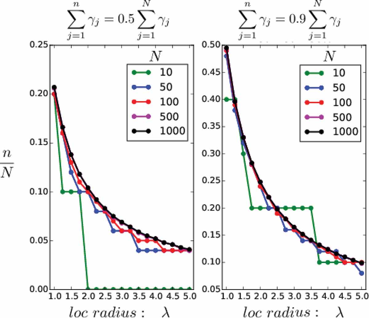
Fig. 9.
Construction of in SC and WC4DEnVar. For different number of grid points and different localisation half widths (horizontal axis), the vertical axis shows the ratio of retained eigenvalues over , in order to cover a given fraction of the total sum of eigenvalues. For the left panel this fraction is , in the right panel it is .