
Table 1.
Overview of a set of 251 pre-selected sounding channels before further selection based on DFS. The frequencies and represent the minimum and maximum frequency of each spectral interval that is uniformly discretised with BW
+ ICI315.15335.15100021ICI416.76432.76100017None440.00456.00100017ICI
Table 2.
Overview of the 25 pre-selected window channels with their corresponding bandwidth. Information is given on the current and future availability of the channels displayed in the list with examples of current and planned (marked with an asterisk) sensors
[i] Note: GMI = GPM Microwave Imager; GPM = Global Precipitation Measurement
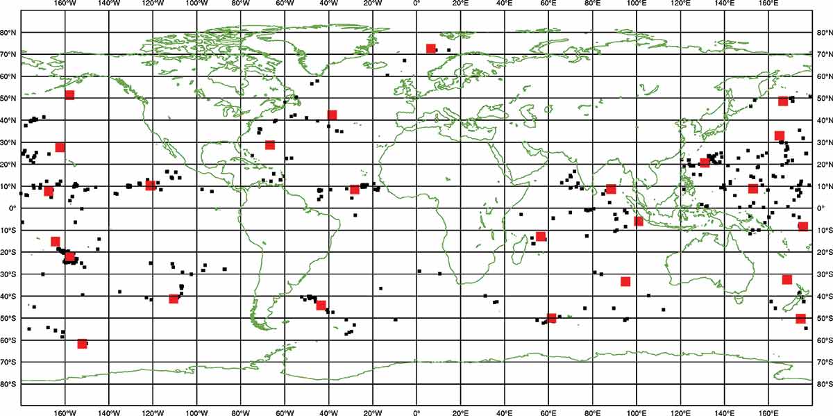
Fig. 1.
Set of 613 profiles over oceans taken from an ECMWF 48 h forecast starting on 10 July 2006 small (black squares). The large red squares indicate the location of the 25 selected profiles.
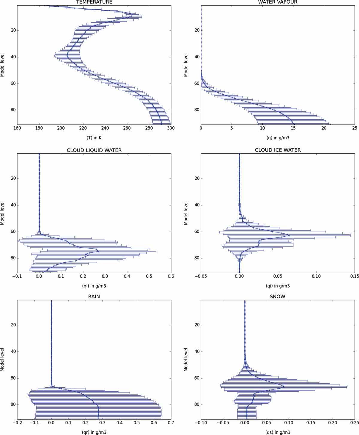
Fig. 2.
Mean and standard deviation of the 25 profiles of the database for temperature (a), water vapour (b), cloud liquid water (c), cloud ice water (d), rain (e) and snow (f).
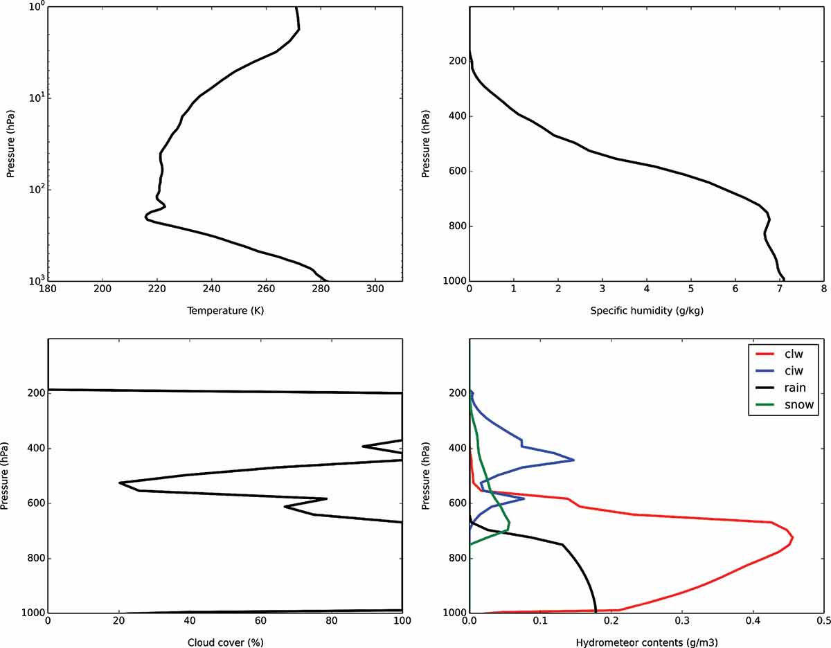
Fig. 3.
Temperature (a), water vapour (b), fractional cloud cover (c), hydrometeor contents (d) for the 13th profile of the database.
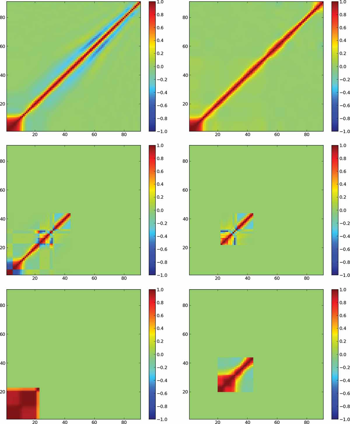
Fig. 4.
Correlation of background errors for temperature (a), water vapour (b), cloud liquid water (c), cloud ice water (d), liquid precipitation (e) and solid precipitation (f) for the 13th profile of the database.
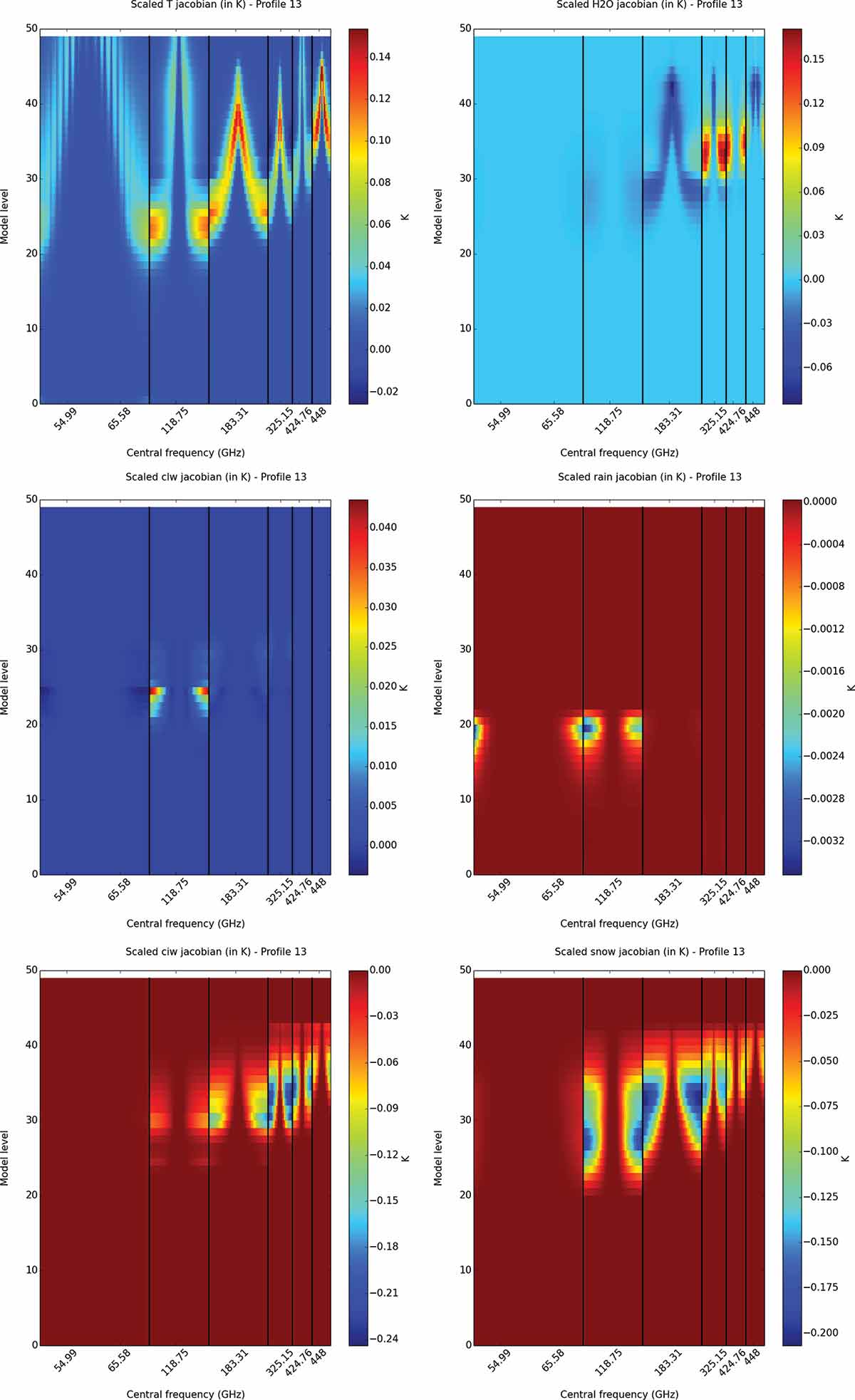
Fig. 5.
Scaled Jacobians in K for cloud liquid water (a), liquid precipitation (b), cloud ice water (c) and solid precipitation (d) for the 13th profile of the database in oxygen and water vapour absorption bands (see Table 1).
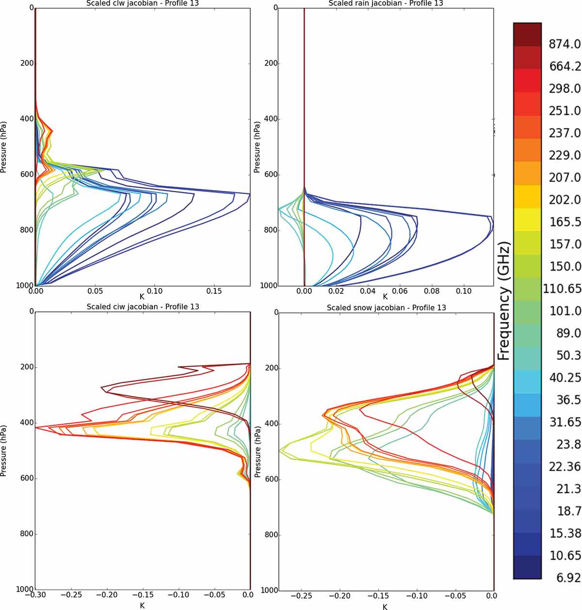
Fig. 6.
Scaled Jacobians in K for cloud liquid water (a), liquid precipitation (b), cloud ice water (c) and solid precipitation (d) for the 13th profile of the database in window regions (see Table 2), over ocean surface.
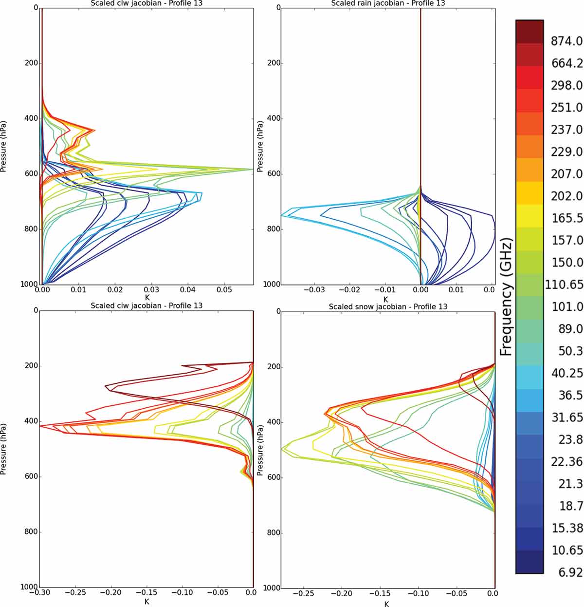
Fig. 7.
Scaled Jacobians in K for cloud liquid water (a), liquid precipitation (b), cloud ice water (c) and solid precipitation (d) for the 13th profile of the database in window regions (see Table 2), over land surface.
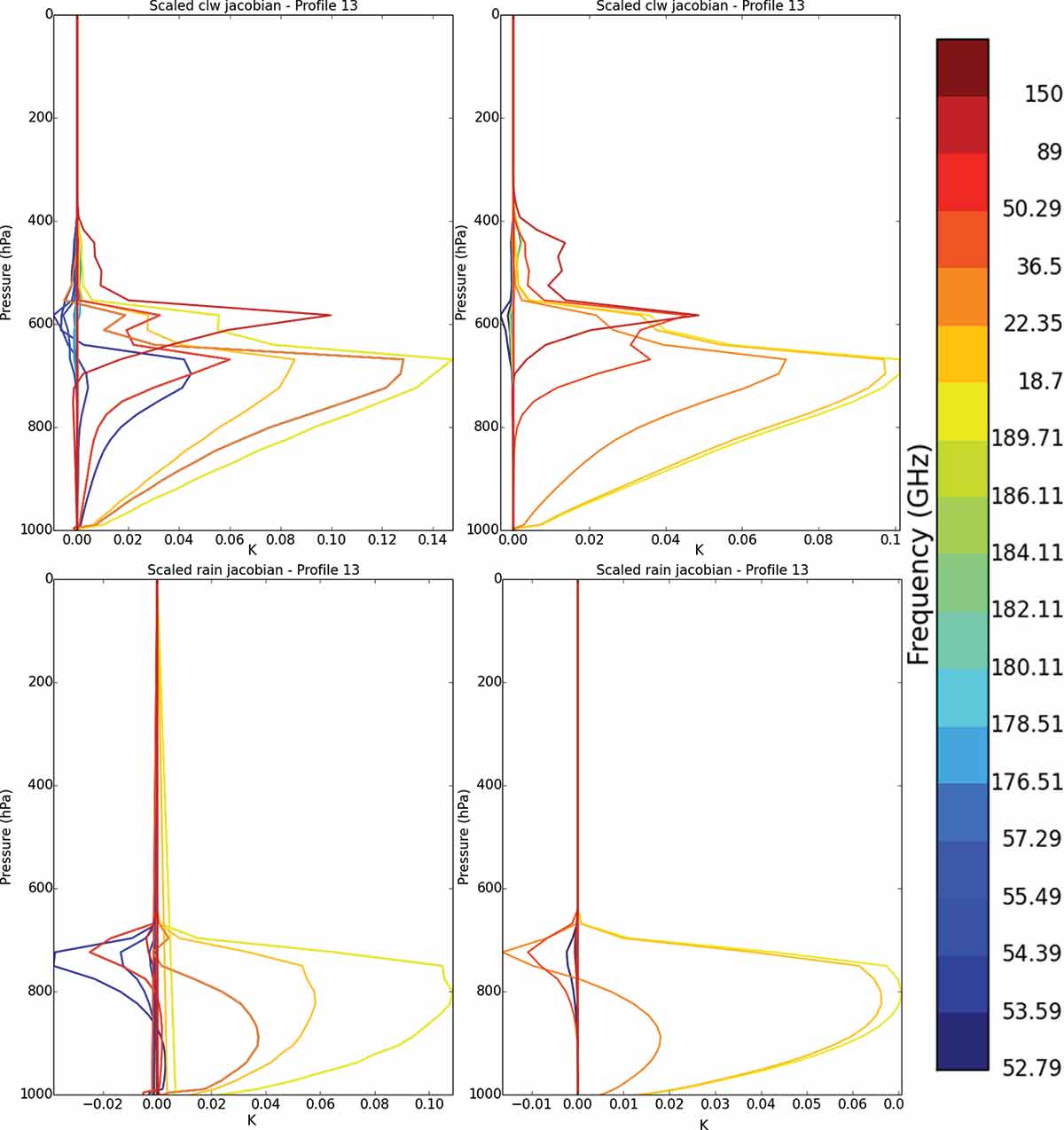
Fig. 8.
Comparison of scaled Jacobians in K for cloud liquid water (top) and rain (bottom) between SSMI/S computed with RTTOV-SCATT (left column) and SSMI/S ‘surrogate’ computed with ARTS (right column) for the 13th profile of the database (set of 18 sounding and window channels between 18.7 and 183 GHz).
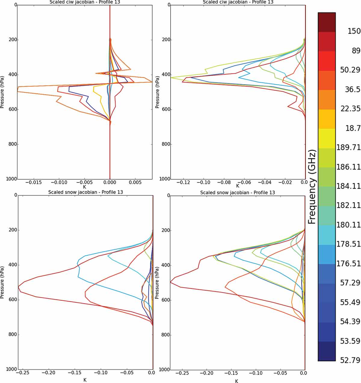
Fig. 9.
Comparison of scaled Jacobians in K for cloud ice water (top) and solid precipitation (bottom) between SSMI/S computed with RTTOV-SCATT (left column) and SSMI/S ‘surrogate’ computed with ARTS (right column) for the 13th profile of the database (set of 18 sounding and window channels between 18.7 and 183 GHz).
Table 3.
Summary of the ten most informative channels on cloud liquid water , liquid precipitation , cloud ice water and solid precipitation for a microwave radiometer spanning frequencies between 6.9 and 200 GHz with a 53° incidence angle over oceans for a set of 25 constrated profiles, together with the corresponding fractional DFS, over ocean surfaces. This configuration is similar to the experimental set-up of DMB2006. The frequencies in bold are not available on current or future instruments. Other frequencies are available on current and future instruments, in italic for window regions and in roman for absorption band
Table 4.
Same as Table 3 over land surfaces
Table 5.
Summary of the twenty most informative channels on cloud liquid water , liquid precipitation , cloud ice water , solid precipitation , specific humidity q and temperature T for an HYMS instrument spanning frequencies between 6.9 and 874 GHz with a 53° incidence angle over oceans for a set of 25 constrated profiles, together with the corresponding fractional DFS, over ocean surfaces. The frequencies in bold are not available on current instruments. Other frequencies are available on current and future instruments, in italic for window regions and in roman for and absorption bands
Table 6.
Summary of the microphysical properties of the various experimental set-ups. The particule size distributions are defined as: H98 (Hess et al., 1998), MP48 (Marshall and Palmer, 1948), MH97 (McFarquhar and Heymsfield, 1997), MGD (Modified Gamma Distribution), F07 (Field et al., 2007). For non-spherical particles, the ‘sector snowflake’ is chosen for the Liu-DDA and the ‘aggregate’ for the Hong-DDA
Liu-DDA ≤ 89 GHz and Hong-DAA > 89 GHz for qs (F07)mix 2Mie spheres for ql (MGD), qr (MP48), qi (MGD)
Liu-DDA ≤ 183 GHz and Hong-DAA > 183 GHz for qs (F07)mix 3Mie spheres for ql (MGD), qr (MP48), qi (MGD)
Liu-DDA ≤ 340 GHz and Hong-DAA > 340 GHz for qs (F07)
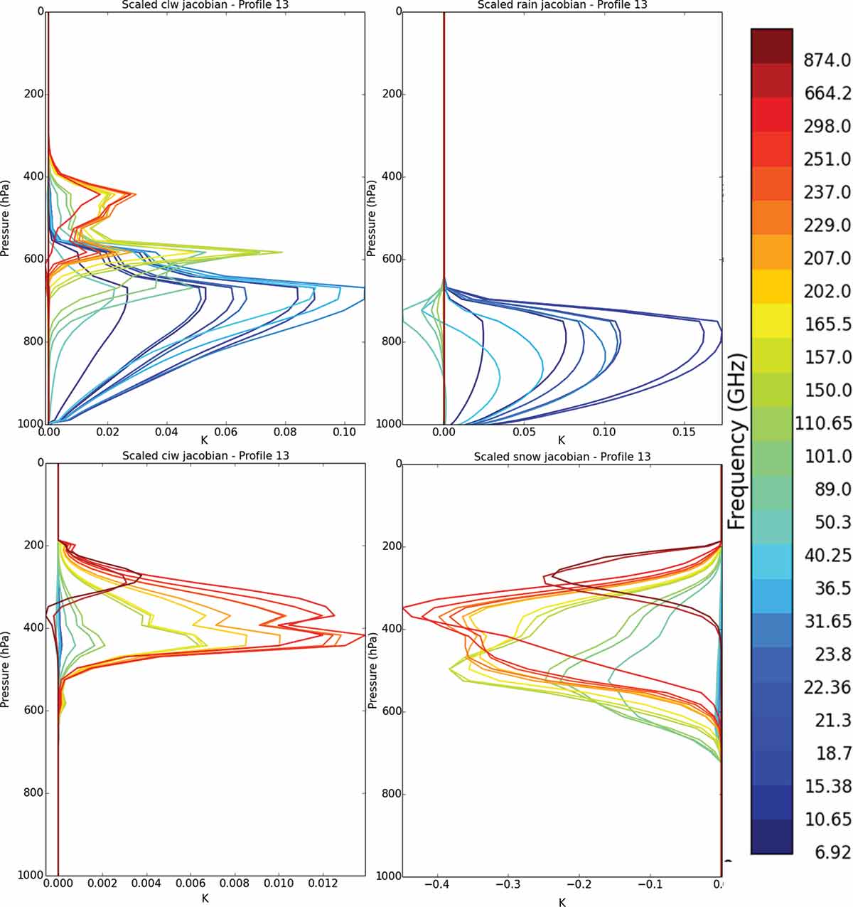
Fig. 10.
Scaled Jacobians in K for cloud liquid water (a), liquid precipitation (b), cloud ice water (c) and solid precipitation (d) for the 13th profile of the database in window regions (see Table 2), for ‘mix1’ set-up over ocean surface.
Table 7.
Summary of most informative channels on cloud liquid water , liquid precipitation , cloud ice water , solid precipitation , specific humidity q and temperature T for an HYMS instrument spanning frequencies between 6.9 and 874 GHz with a 53° incidence angle over oceans for a set of 25 constrated profiles, for a set of four microphysical properties summarised in Table 6
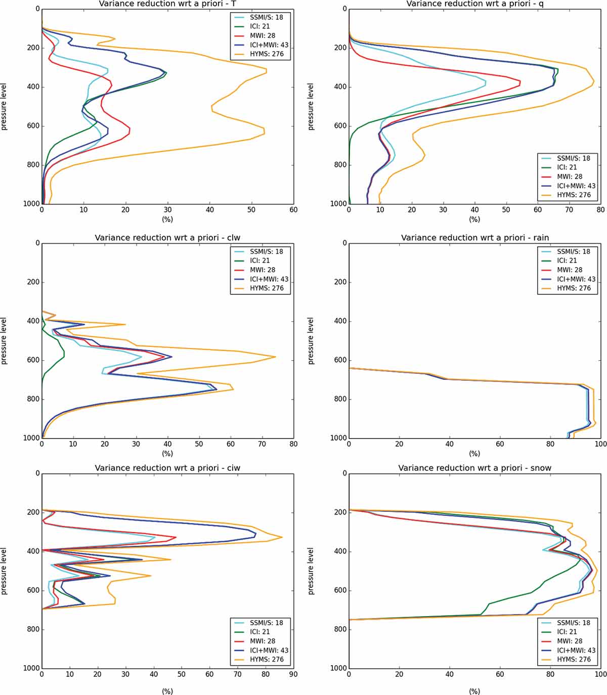
Fig. 11.
Variance reduction (expressed in percentage) for temperature (a), water vapour (b), cloud liquid water (c), cloud ice water (d), liquid precipitation (e) and solid precipitation (f) induced by the assimilation of SSMI/S, MWI, ICI, MWI + ICI and HYMS microwave instruments for the 13th profile of the database and the ‘all’ set-up for microphysics.
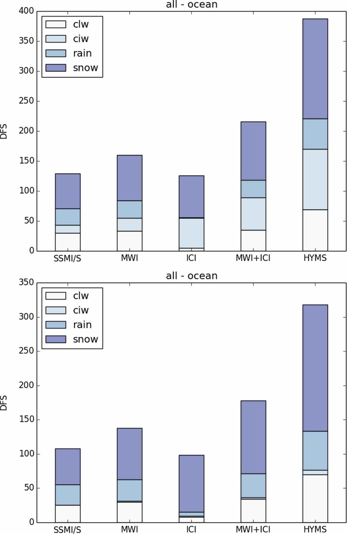
Fig. 12.
Degrees of Freedom for Signal (DFS) for the following hydrometeors: cloud liquid water (clw), cloud ice water (clw), liquid precipitation (rain), solid precipitation (snow). They are given for various configurations of present and future microwave radiometers, for ‘all’ (top panel) and ‘mix1’ (bottom panel) set-ups. Each DFS has been computed over a set of 25 atmospheric profiles. The corresponding microphysical properties are summarised in Table 6.