
Table 1.
Overview of the locations for the HOBO rain gauges (P1–P12) and the meteorological stations (denoted by their national code)
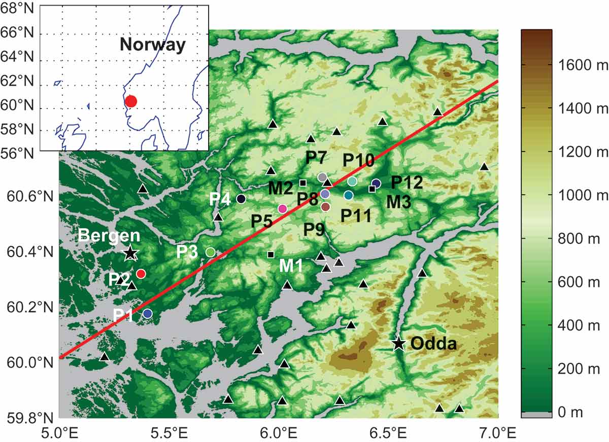
Fig. 1.
Map of the experiment area with altitude from the terrain database ASTER GDEM v1 (Tachikawa et al., 2011) contoured in colours. The deployed rain gauges are colour coded and the stations P1–P12 correspond to the line colours in Fig. 5. Black squares are the stations M1–M3 referenced in the text, triangles are the remaining precipitation stations in the area operated by the Norwegian Meteorological Institute (MET Norway). The red line shows the lower edge of the cross sections analysed in Section 3.4.
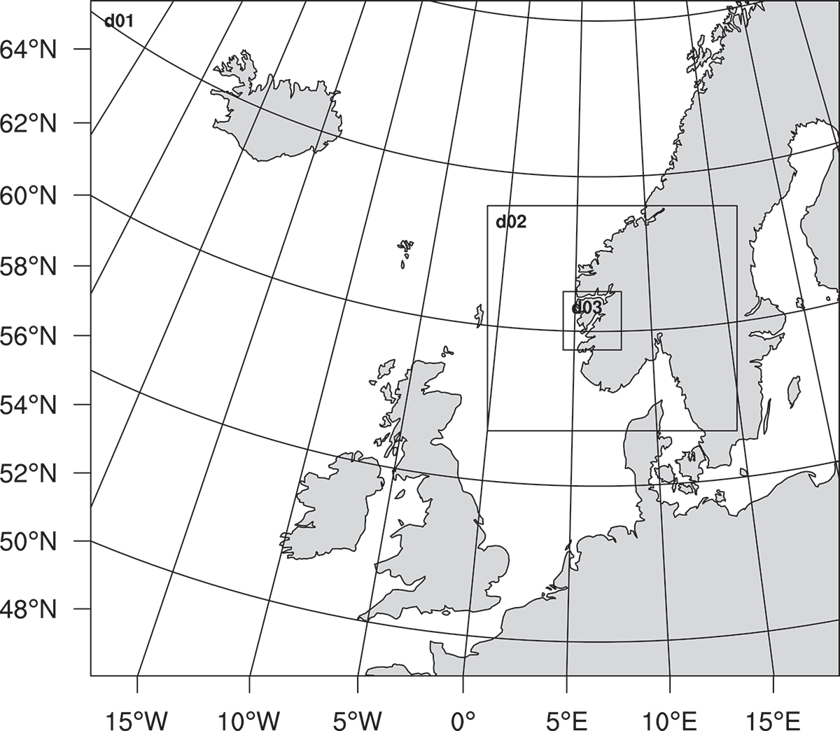
Fig. 2.
Model domain set up for the WRF simulations. The domains d01, d02 and d03 have horizontal grid resolutions of 9 km, 3 km and 1 km, respectively.
Table 2.
Overview of the physical parametrisation schemes used in the WRF simulations
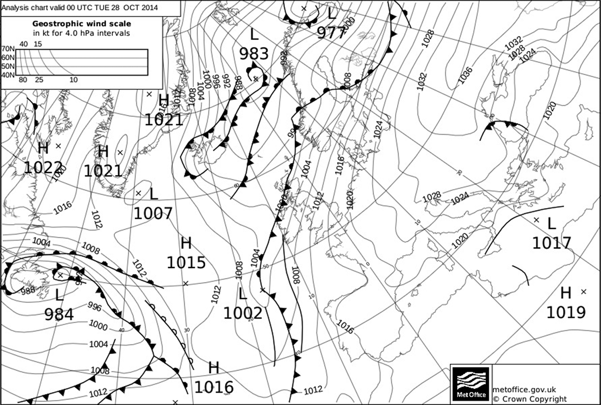
Fig. 3.
Surface analysis chart from UK Meteorological Office, for 28 October 2014 00 UTC. Reproduced with kind permission of the Met Office.
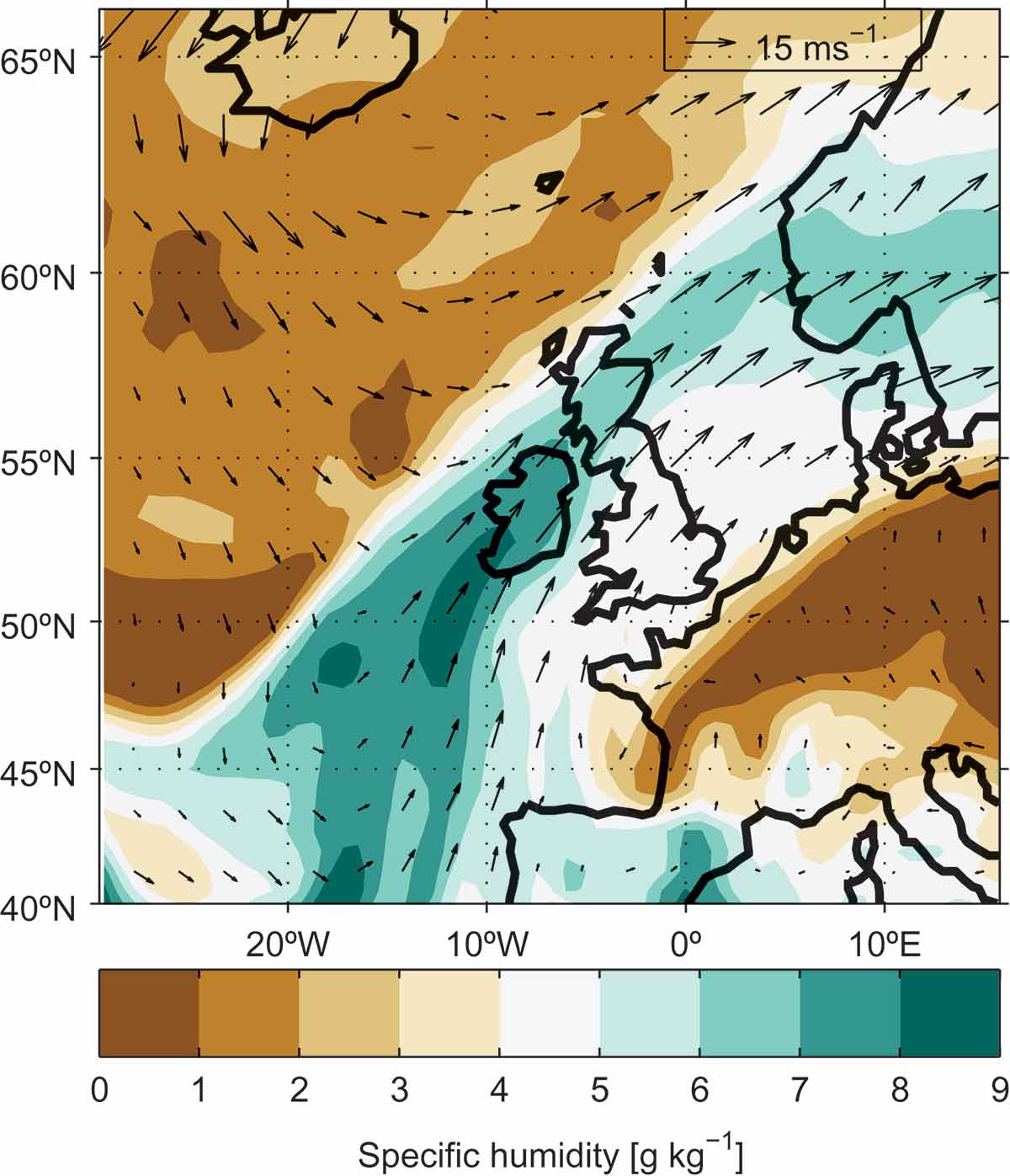
Fig. 4.
Specific humidity (g kg) at 850 hPa at 00 UTC on 28 October (coloured contours) and the 850 hPa wind (arrows). Data from the ERA-Interim reanalysis.
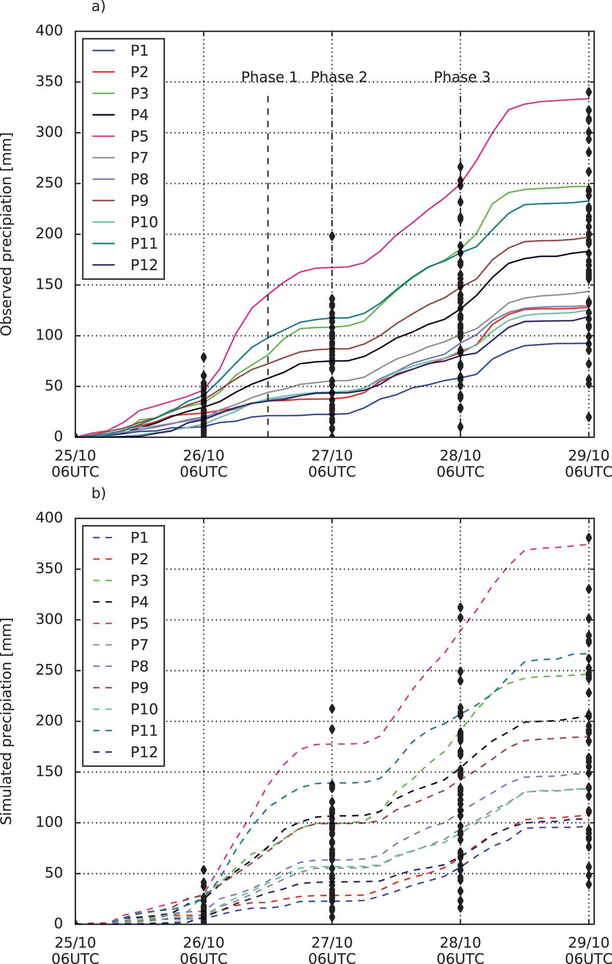
Fig. 5.
The observed (a) and simulated (b) accumulated precipitation amounts during the days before the flooding event, from 25 October 06 UTC to 29 October 2014 06 UTC. The observations of the HOBO rain gauges are given as solid coloured lines and the corresponding results from the interpolated 1 km model simulations as dashed lines. Data from the MET Norway stations are indicated by the black diamonds.
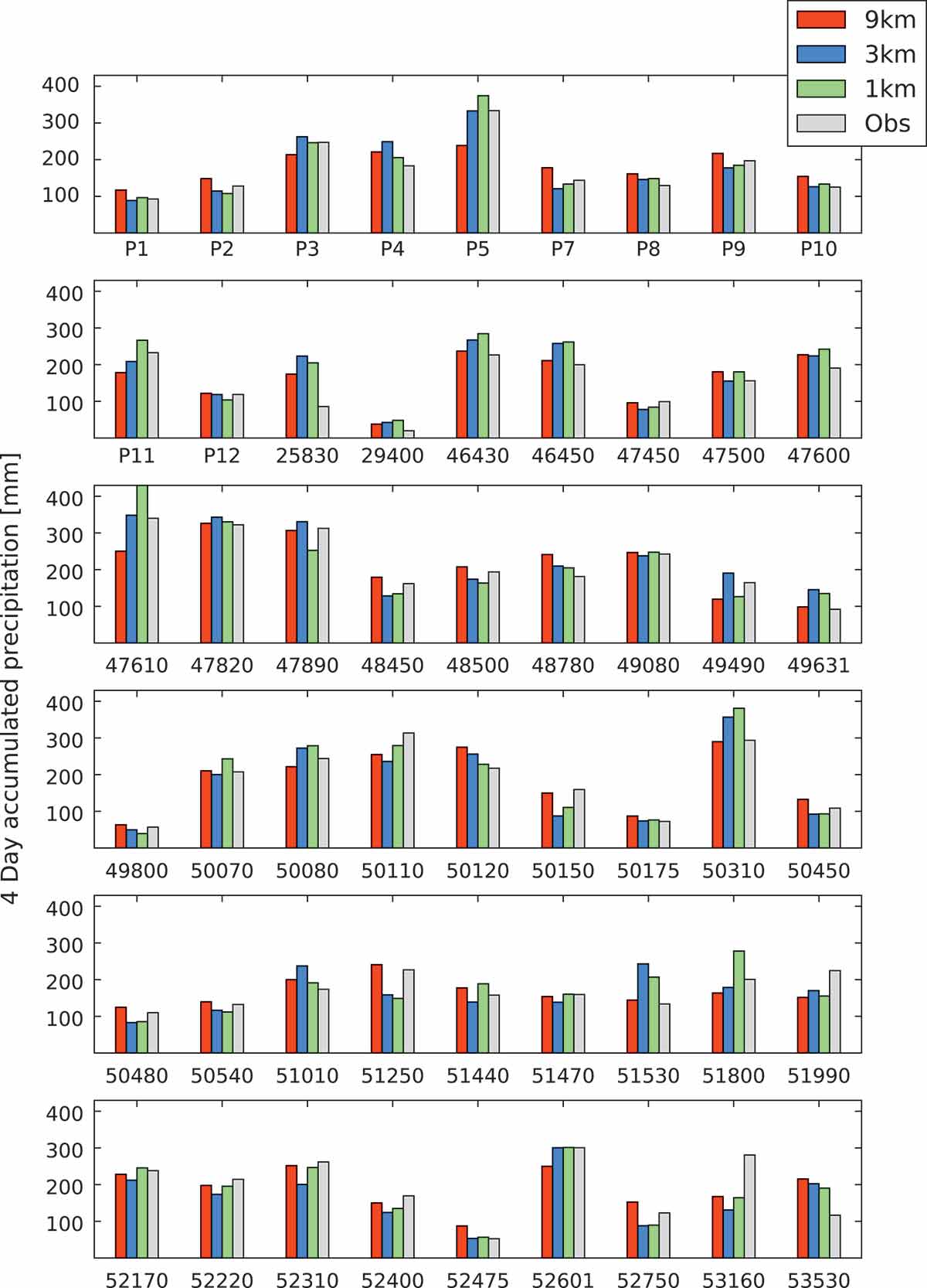
Fig. 6.
Comparison of four-day accumulated precipitation from 25 October 06 UTC till 29 October 06 UTC from the WRF 9 km, 3 km and 1 km model output, using the interpolated grid point, and the observations. There is one set of bars for each station and the labels on the horizontal axis show the station id.
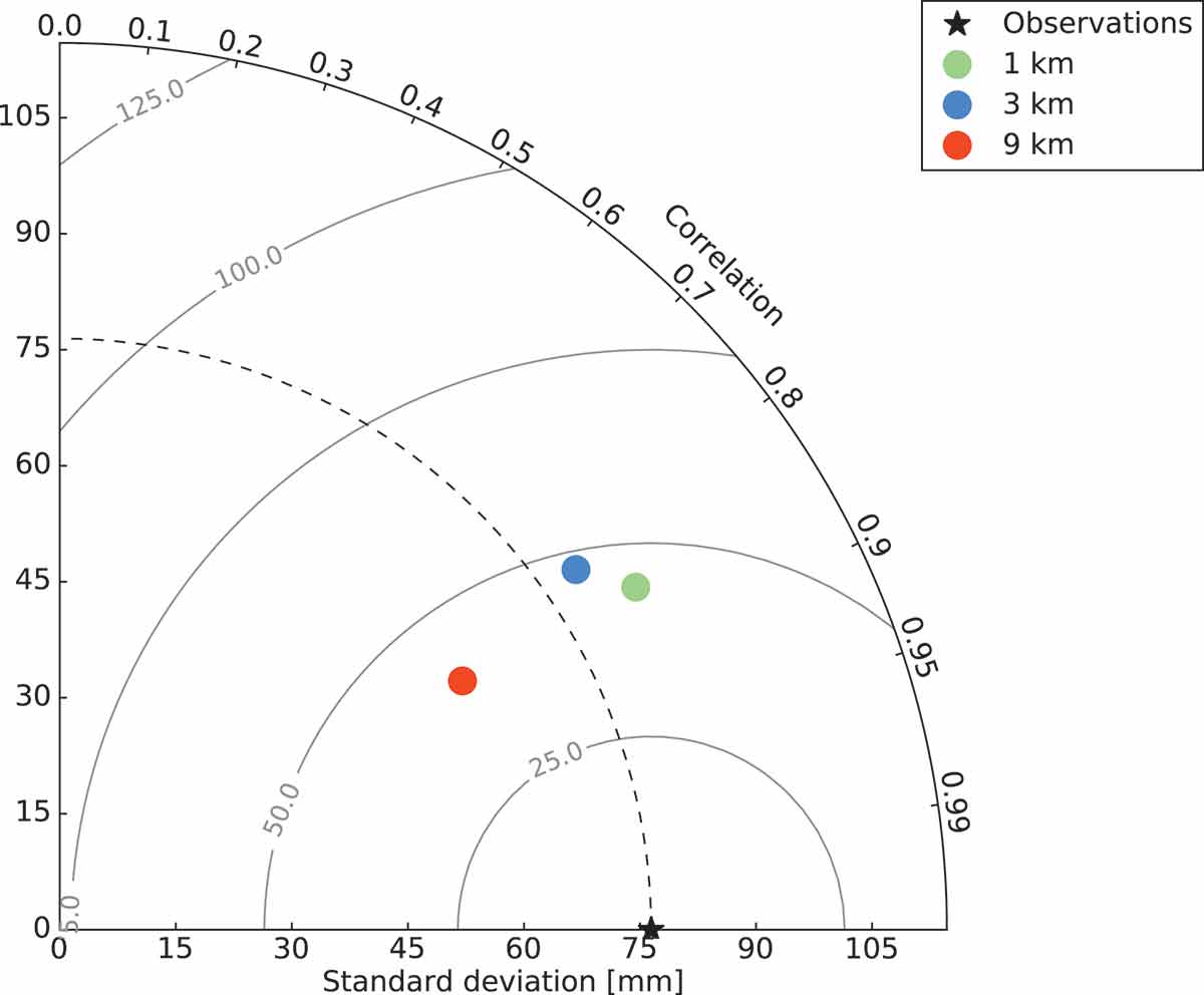
Fig. 7.
A Taylor diagram with the 9 km, 3 km and 1 km simulations marked as circles and the observations marked as a black star for reference.
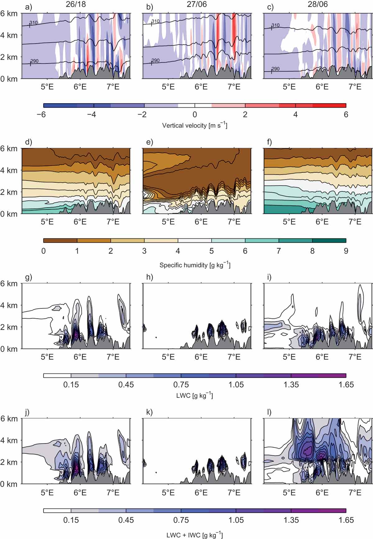
Fig. 8.
Cross sections (above the red line in Fig. 1) of vertical velocities (a–c) with potential temperature contoured in black lines, specific humidity (d–f), liquid water content (g–i) and the sum of liquid and ice water content (j–l) from the 1 km resolution run, at three selected times: 26/18, 27/06 and 28/06 (in the left, middle and right column, respectively).
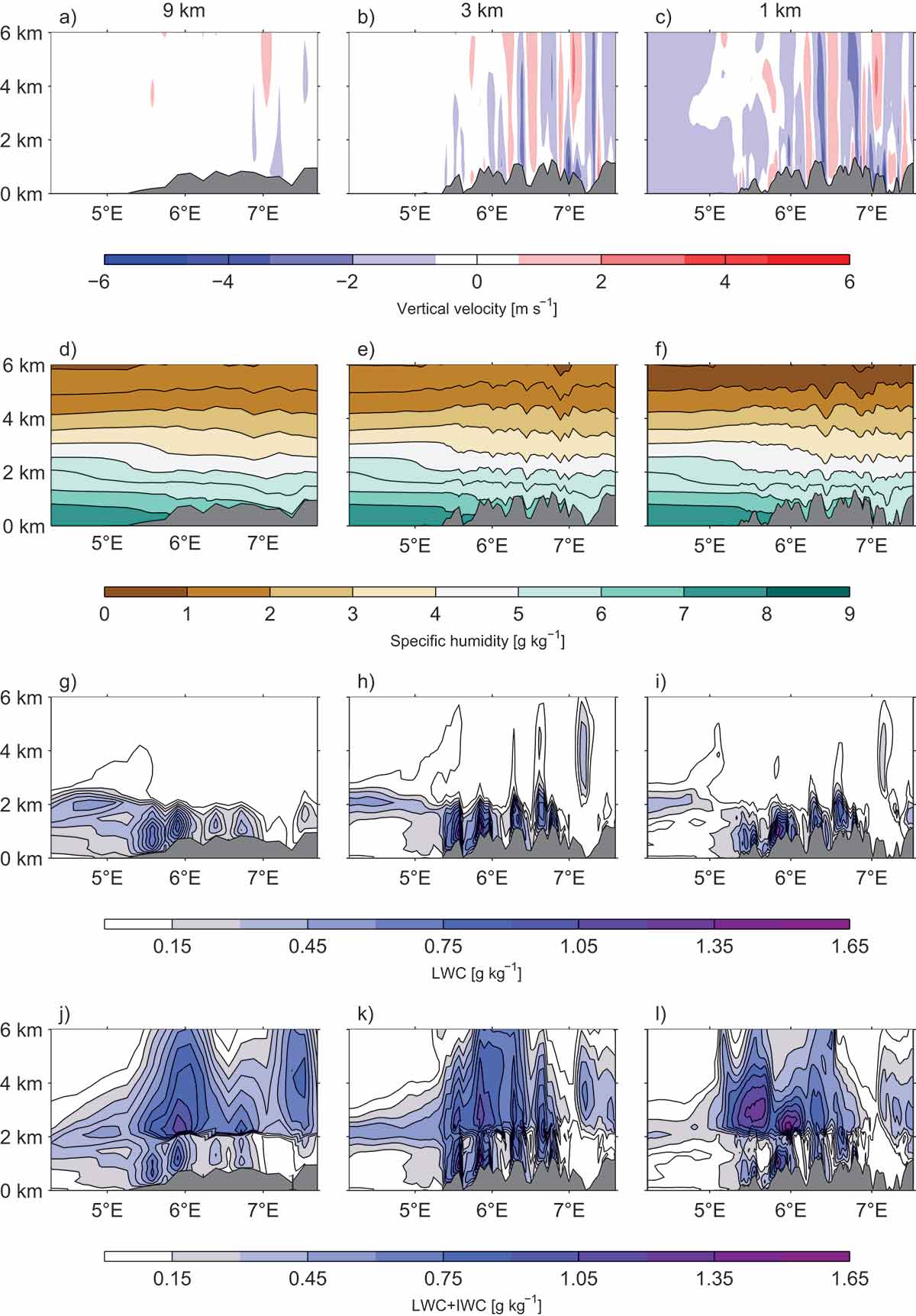
Fig. 9.
Cross sections (above the red line in Fig. 1) of vertical velocities (a–c), specific humidity (d–f), liquid water content (g–i) and the sum of liquid and ice water content (j–l) at time 28/06 for the 9 km, 3 km and 1 km runs (in the left, middle and right column, respectively.
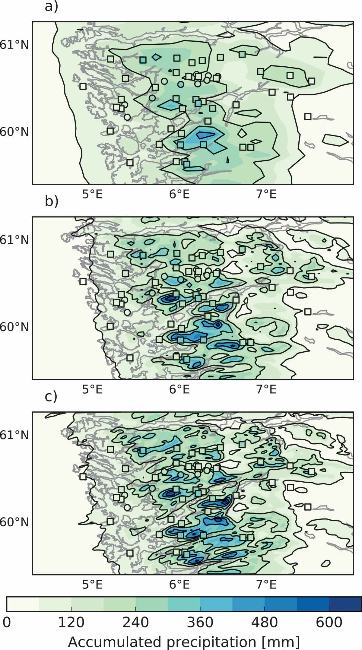
Fig. 10.
Accumulated precipitation (25/06–29/06 October) in part of the 9 km grid (a). The circles correspond to the HOBO stations, squares are stations from MET Norway. The inner parts of the markers show the observed accumulated precipitation amounts in the period. The other panels show the same for part of the 3 km domain in (b) and for the 1 km domain in (c).
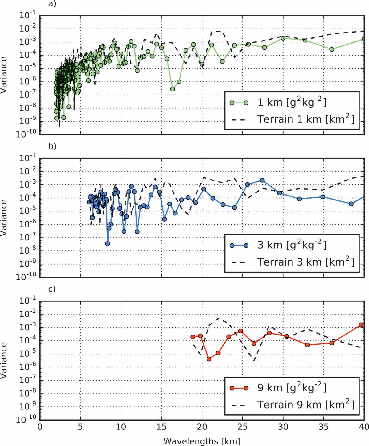
Fig. 11.
The upper panel (a) shows the variance spectrum of the terrain and the specific humidity cross sections (pressure level 850 hPa) shown in Fig. 8 from the 1 km simulations. The middle panel (b) shows the same from the 3 km simulation, and the lower panel (c) for the 9 km simulation.